Selection of the Statistical Model
Our task now is to select a decision model consistent with several levels of policy goals. At the highest level, our model must effectively assist in converting a historical natural-monopoly market to a competitive market. This requires us to ensure that incumbents allow nondiscriminatory access to their infrastructures so competitors can provide local telephone services. That is, the CLEC's customers must not receive significantly worse performance from the ILEC than the ILEC's customers receive. Our decision today is at an even finer level of detail. We must specify a model that will accurately assess and identify discrimination. We must specify accurate calculations, accurate analyses, and accurate discrimination-identification decisions.56
We have reviewed the proposed models and the parties' comments regarding each of these models. While we had hoped that the parties would agree on a model and all the necessary implementation specifications, this did not occur. To the contrary, the parties disagreed on the models and on most of their elements. While the workshop hybrid model57 seemed to come closest to a successful compromise, the parties did not fully endorse it. At best, each party accepted the proposed hybrid model only insofar as we would modify it to address their particular interests.
Thus, we must review and approve or reject proposed models and/or elements, especially to resolve issues where there was no agreement. Unfortunately, virtually all model specifications by each party generated disagreement from at least one other party. The following is a list of the issues we must resolve now to specify the decision model for the next phase of this proceeding.
· Shall we select the workshop hybrid model, or any party's decision model, in its entirety, or should we select the best elements of different models to create a new hybrid?
· What statistical test[s], if any, shall be used to assess parity measures, including average, percentage, and rate measures?
· Where statistical tests are used, what decision criteria shall be used to identify results as parity or non-parity, or in other words, what criteria shall be used to identify test passes and failures?
· Shall a determination of material differences be a factor in non-parity identification?
· What sample size rules should be used?
· Shall data be transformed to closer approximate statistical test assumptions?
· Shall benchmarks be used as limits or as targets, and shall statistical tests, or tables based on statistical analyses, if any, be used for: (1) Some benchmark measures, (2) All benchmark measures?
· Shall correlational analyses be employed to assess and reduce redundancy between performance measures?
· Shall historical data be used as a decision criterion, or be monitored separate from the identification of passes and failures?
· Shall existing benchmarks be modified to address new developments in this assessment phase of the proceeding?
· Should we specify different models for the different ILECs?
· Should we plan to adjust payments retroactively after the six-month trial period?
· What other specifications should we order to enhance the use and understanding of our decision model?
We will base this decision on the following criteria:
· Accuracy: Identify discrimination when it exists, and do not identify discrimination when it does not exist.
· Correctability: When more important criteria do not provide conclusive guides to our decisions, we will select the elements that offer the most opportunity for correction in later phases of this proceeding.
· Academic soundness: Our rationale shall be based on recognized applicable statistical assumptions and principles, and confirmed by data when possible.
· Policy goals: Our rationale will be consistent with competition-enhancing policy and law providing substantially equal access for all potential local phone service providers, whether small or large.
· Simplicity: Without sacrificing higher-order goals such as accuracy, we will prefer the more simple models and elements.
· Fairness: We will strive to be as even-handed as possible to optimize competitive market potential and benefits.
· Openness: We will document and explain the criteria we use in selecting the model and its elements so that all parties can knowledgeably comment and knowledgeably argue for modifications to the model.
· Consensus: We will prefer models or elements where a consensus exists, unless there are differences on more important criteria.
· Experimentation: Rather than consider the initial model to be a final product, we will consider this initial implementation to be an experiment that will inform future model development.
· Costs: Unless a more costly model or element is likely to better satisfy important criteria, we will prefer less costly approaches.
· Understandability: When differences on more important criteria are minimal, we will prefer more easily understandable models and elements. We will also take care to explain models, elements, and analyses in sufficient detail and at a level to help the reader understand the model we specify and the reasons we have selected the model and its elements.
From the parties' proposals and comments, relevant statistical sources, and staff's analyses, using the above criteria we have selected a decision model.58 The model is presented in Appendix C. The following is a discussion of the model and our rationale for selection of the various model elements.
Decision accuracy
While the above criteria lists may seem self-explanatory, we believe it important to discuss at length the first and most important criterion, decision accuracy. We begin with a brief overview.
Once performance measures are established and results are obtained, accurately assessing the existence of competitive conditions then becomes a decision-making task. Since these decisions must be self-executing, the Commission must construct a decision model that can automatically identify performance result levels that reveal competition barriers and that will trigger incentive payments. There are two fundamental categories of performance measures that must be assessed. These categories' definitions are based on the characteristics of the service an ILEC provides a CLEC and the CLEC's customers. Where there is an ILEC retail analogue to the service given the CLECs and their customers, the FCC has stated that parity of services is evidence of open competition.59 Where there is no ILEC retail analogue to service given the CLECs, then open competition is gauged by performance levels that provide a "meaningful opportunity to compete."60 These performance levels that have no retail analogue are designated "benchmarks." Thus, the two categories of measures have been termed "parity" and "benchmark" measures.
Decisions regarding parity measures
In identifying parity or non-parity, accurate remedies-plan decision-making is not simply a matter of accurately calculating average ILEC and CLEC performance and identifying non-parity if ILEC service to CLEC customers is worse than ILEC service to ILEC customers. Given that there is variability in ILEC performance in its own retail services to its own customers, a measurement result of inferior service to CLEC customers could be due either to this variability, or actual discrimination, or both. In other words, if we sample the ILEC's service results to its own customers, we will get different results, some better, some worse than the average. Service to a CLEC may be viewed as a "sample" of the ILEC's services.61 Theoretically speaking, if the performance measured from the CLEC "sample" is typical of the performance for similar ILEC customer "samples," then there is no evidence of discriminatory service, even if it is somewhat worse than the ILEC average. However, if the CLEC "sample" performance is worse than most ILEC customer "samples," then there appears to be evidence of discrimination.
In statistical terminology, the non-discriminatory variability between multiple ILEC samples is termed "sampling error" or "unsystematic variability," referring to the fact that the variability is simply due to random sampling outcomes. Discriminatory variability is the case where the performance in a CLEC sample is worse than what would be reasonably expected from sampling error. Discriminatory variability is variability that goes beyond sampling error and is termed "systematic variability," meaning that something is systematically causing the differences between the samples. Since these two types of variability cannot be directly observed, discrimination or non-discrimination must be indirectly inferred.
A decision outcome matrix illustrates this problem. Figure 1 presents the four possible decision outcomes about parity. The four outcomes represent conclusions of either parity or non-parity of service under conditions of either actual parity or non-parity. The decision outcome matrix simply recognizes that when we make a dichotomous decision, there are four possible outcomes, two correct and two incorrect. In the context of this proceeding, the decision outcome matrix illustrates decision goals: (1) to detect differences when they exist, and (2) to not detect differences when they don't exist.
Figure 1: Decision Matrix
Parity Identified Non-Parity Identified
(Decision: No Discrimination) (Decision: Discrimination)
|
Reality: Parity (No Discrimination) |
(True Negative) |
(False Positive) |
|
Reality: Non-Parity (Discrimination) |
(False Negative) |
(True Positive) |
Figure 2 expands this illustration. Given that decisions regarding parity are based on measurements that are comprised of both "true" values and "error," these outcomes can represent both correct and incorrect decisions, depending on the relative amount of error in the measurement. Figure 2 portrays sampling error effects.
Figure 2: Decision Matrix Showing Sampling Error Effects
Decision: Parity Decision: Non-parity
|
Reality: Parity (No discrimination) |
Correct Decision Relatively low sampling error |
Incorrect Decision Sampling error creates spurious difference |
|
Reality: Non-parity (Discrimination) |
Incorrect Decision Sampling error masks real difference |
Correct Decision Relatively low sampling error |
Figure 3 illustrates the contribution of statistical testing. The potential for errors is the same as in the first two matrices where no statistical testing is applied. The only contribution of statistical testing is that it allows us to estimate decision accuracy, or in other words, to calculate the decision error probabilities. These probabilities can then assist decision-making by quantifying the different error probabilities and comparing them to standards of confidence that we wish to apply. These standards of confidence are expressed as: (1) the power of the test, and (2) the confidence level.
Figure 3: Decision Matrix with Statistical Tests
Decision: Parity Decision: Non-parity
|
Reality: Parity (No discrimination) |
Confidence level Probability = 1 - alpha |
Level of significance Probability = alpha Type I error |
|
Reality: Non-parity (Discrimination) |
Test insensitivity Probability = beta Type II error |
Test power or sensitivity Probability = 1 - beta |
Test power refers to the ability of the test to actually find true differences, that is, the confidence that you found what you were looking for, when it existed. "Confidence level"62 refers to the ability of the test to reject spurious differences, that is, the confidence that when you identified something, it actually existed. Together, these probabilities represent the amount of confidence one can have in decision quality. The higher the test power, the greater the confidence one can have that true differences were uncovered. The higher the "confidence level" the greater confidence one can have that discovered differences are real differences. Other things being equal, as one level of confidence is increased, the other decreases. In other words, the more powerful the test, the more likely there will also be differences found solely due to random variation, and the higher the confidence level, the more likely true differences will be missed. Neither confidence standard is inherently more important than the other. Each application of a statistical test implies different trade-offs between these two confidence standards, and their corresponding error probabilities, depending on the consequences of the two different errors.63
In the present case of restructuring a historical natural-monopoly market to create a competitive market, the primary function of performance measurements and the decisions about performance measurements is to detect and prevent barriers to competition. To maximize goal attainment these decisions must be as accurate as possible, to find and prevent actual barriers, and to avoid identifying barriers when they do not exist. However, there is no legislative or regulatory guidance specifying the relative importance of the two decision errors.
On one hand, if we do not detect barriers when they occur, competition may fail, and the fundamental purpose of the legislation will have been thwarted. On the other hand, if we identify barriers when they do not exist, then we are likely to take unfair punitive action. Therefore we will use statistical testing to assess the balance between these two competing outcomes, thus enabling greater decision quality and attainment of legislative goals. Figure 4 summarizes the statistical decision matrix and identifies the probabilities that correspond to the four possible decision outcomes.
Figure 4: Decision Matrix Statistical Testing Summary
Decision: Parity Decision: Non-parity
|
Reality: Parity |
No barriers exist. No barriers identified. (1 - alpha) |
No barriers exist. Barriers identified. (alpha) Type I error |
|
Reality: Non-parity |
Barriers exist. No barriers identified. (beta) Type II error |
Barriers exist. Barriers identified. (1 - beta) |
Using measures of performance averages and variability, statistical analysis provides estimates of: (1) the probability that a result of a certain magnitude would be detected when it exists (test power and corresponding error beta) and (2) the probability that the result is due to random variation when in fact there are no differences (confidence level and corresponding error alpha). The methodology for using these estimates to establish dichotomous decision criteria is called null hypothesis significance testing. The analyst specifies a null hypothesis to pose that there are no differences between two performance outcomes, selects a confidence level that strikes the appropriate balance between the two types of error, calculates the probabilities, and compares them to the selected significance level. If the probability is less than the selected significance level, then the analyst rejects the null hypothesis and accepts the alternative hypothesis that there are real differences.
In the two approved Section 271 applications to date, Bell Atlantic New York and Southwestern Bell in Texas use a "Z-test" statistic to calculate these probabilities. Conceptually, the Z-test statistic compares the ILEC's average (mean) performance to the CLEC's mean performance, and then compares the difference between the means to the difference that would be expected from random variation at a selected confidence level. The expected difference is calculated from the variability in the samples of performance. The greater the variability, the greater the expected difference, and the less likely a true difference will be detected. In the Z-test, the difference between means is compared to (actually divided by) an expected difference term that is calculated from the sample size (n) and the variability in those samples (variance).
Thus the sample size, the variability in the samples, the power of the test, the confidence level, and the size of the true differences between means affect decision quality.64 These elements are interdependent such that changing one will have an unavoidable effect on at least one of the others. A convention has existed for several decades to pre-select a fixed confidence level (or alpha) and adjust the other elements if desired. For example, if a test with the common 95% confidence level (0.05 alpha) lacked adequate power to detect true differences, the sample size could be increased. Methods have been developed to calculate the minimum sample size required to attain adequate test power.65
Additionally, since much of science depends on replication, test power is relegated less attention because of the expectation that experiment replication will address this issue. However, this convention which evolved in the 1920's, called null hypothesis significance testing, has been questioned over the last three or four decades. At least one professional standards board was recently established to consider abandoning such testing in favor of new methods that strike a more even balance between test power and confidence levels.66 Illustrating this concern about ignorance of test power, the following comments reveal some of the intense dissatisfaction with current research relying on 0.05 critical alpha levels:
Whereas most researchers falsely believe that the significance test has an error rate of 5%, empirical studies show the average error rate across psychology is 60%--12 times higher than researchers think it to be. The error rate for inference using the significance test is greater than the error rate using a coin toss to replace the empirical study. . . . If 60% of studies falsely interpret their primary results, then reviewers who base their reviews on the interpreted study "findings" will have a 100% error rate in concluding that there is conflict between study results. (p. 3.)67
The balance between these interdependent elements that affect decision outcome quality is problematic not only in pure research contexts, but also in applied contexts such as engineering and operations management.68 As parties have greater vested interests in different outcomes, the greater the argument there is over the appropriate balance. This is certainly the case in the present proceeding. Parties disagree on what is appropriate for all elements: the appropriate tests, confidence level, test power, sample size, test statistic, and other elements and nuances of a statistically based decision structure.
Determinations regarding benchmarks
Unlike performance measures where there is a retail analogue, benchmarks cannot compare ILEC service to CLEC service since there is no ILEC service analog. Instead, benchmarks are judgments about the levels of ILEC performance for CLEC competitive service that are necessary to "allow a meaningful opportunity to compete." Benchmarks have been constructed as tolerance limits. For example, one measure specifies that 99 percent of billing invoices shall be available within 10 days of the close of the billing cycle.69 The issues for statistical analysis accuracy are not the same as for parity measures. However, small sample benchmark applications raise similar decision matrix issues that we discuss after we address the more complex issues of the statistical models for parity performance measurement results.
Statistical models
As discussed, several models for parity assessment have been presented during the course of this proceeding. Some were intended to be complete, such as Pacific's most recent model. Other models were intended to present conceptual frameworks that would resolve various problems and which could be implemented with further negotiation and development. Examples of these include ORA's model, MCI's SiMPL model, and the ACR's proposal. We find that none of the presented models are acceptable in their entirety. Our rationale for this finding is best explained by discussing our evaluation and selection of the model elements that we will specify in what will be a new "hybrid" of elements from each of the different models presented in this proceeding.
Statistical tests
Three types of parity measurements have been developed for monitoring ILEC performance: averages, percentages, and rates. Each measurement type requires a different statistical test or a variant of the same test.
Average-based measures
The choice of a statistical test for average-based parity measures came as close as any model element to being accepted by all parties. Pacific and the CLECs have agreed that the Modified Z-test should be applied to average-based measures. Verizon CA also agreed to use the Modified Z-test, albeit with modifications. Only ORA disagreed, although they consented to its use in the development of a "hybrid" model. (RT at 1103.) All parties have agreed that a one-tailed test should be used. A one-tailed test is appropriate for situations where we are only interested in outcomes in one direction, in this case where the CLEC performance results are worse than the ILEC results. This is consistent with academic texts70 and with the FCC's view of the appropriate statistical application regarding the requirements of the Act.71
Standard Z-test
The standard Z-test compares the difference between means to what is essentially an expected difference between means that could be explained by random variation. The expected difference is calculated from the variation (variance) in both the ILEC and CLEC results. The ACR proposed that the ILEC and CLEC variances be screened for statistically significant differences as a first step, then either the pooled or equal variance standard Z-test statistic would be calculated as a second step depending upon the results of the first step. Verizon CA described several concerns with the ACR's proposed two-step standard Z-test method and suggested several corrections.72 However, in response to the CLECs' concerns that ILEC discrimination could increase the CLEC variance, and thus make it more difficult to detect any discrimination, all parties agreed to use a Modified Z-test instead of the standard Z-test.
Modified Z-test
This test was first adopted by the NYPSC for the BANY 271-application performance remedy plan.73 Similar to our situation, since the CLECs were concerned that by providing highly variable service to the CLECs, the ILEC theoretically could increase the expected difference and thus mask real differences, the parties in the BANY application proceedings agreed that the CLEC variance would not be part of the expected difference calculation. This alteration has been given the name "Modified Z-test." The FCC considers this test reasonable,74 and it has been favorably presented in statistical academic literature.75 The FCC subsequently approved Southwest Bell's performance remedy plan for Texas, which also uses the Modified Z-test.76
Only ORA objects to use of the Modified Z-test, although for the purposes of developing a hybrid model, ORA is willing to proceed using the test. (RT at 1103.) ORA's primary concern is based in their opinion that use of any Z-test requires that the data be normally distributed. According to the statistical literature, this may be only partially correct; Central Limit Theorem states that for large samples, non-normality in the data does not affect the test.77 With large samples, the distribution of sample means will be normal, whether or not the raw data distribution is normal. The means of sample sizes of 30 or more are typically considered sufficiently normally distributed to have minimal effect on a Z-test.78 The BANY performance remedy plan addresses this issue by using the Modified Z-test down to a sample size of 30, and is temporarily using the t-test for smaller samples until permutation testing is established.79
Verizon CA agrees to use the Modified Z-test, although its agreement is conditional. Most importantly, Verizon CA agrees to use the Modified Z-test for average-based measures if a permutation test is used for small samples. As discussed below, we agree with the concept, but have concerns with the implementation.
Permutation tests
To remedy the problem of small samples, which may not meet the "normality" assumptions of the Modified Z-test, Verizon CA proposed that a permutation test be used for average-based and other performance measures. The permutation test is a statistical test that, independent of any underlying distribution, assesses the probability of an outcome. As such it is termed a "distribution free" or non-parametric test in contrast to the parametric Z-test which is based on distribution assumptions.80 The reasoning behind its use is that when the Z-test normality assumption is violated, a permutation test is more appropriate and accurate since it compares the actual CLEC data directly to the ILEC data without making distribution inferences. Theoretically, the test is only necessary for smaller samples where Central Limit Theorem does not predict normality, because the two tests should produce similar results for larger samples. Differences in distributions do not affect permutation test results, and "look-up" distribution tables, such as "Z" or "t" tables are not necessary.81 In theory, the benefit of permutation testing is that it can increase the accuracy of the error estimates, thus enabling more accurate decisions.
Only Pacific objects to the use of permutation tests.82 Pacific originally objected to the assumed costs of such a procedure, but continues to object even though those costs have turned out to be much smaller than originally assumed.83 Pacific now objects to the procedure as being inadequately tested and too complex,84 although earlier had acknowledged its feasibility at least for Pacific samples less than 5,000 or 10,000.85 Regarding the feasibility of its use for such large samples, Verizon CA has presented procedures for implementing permutation on samples of any size.86
The selection of the appropriate test for small samples should be based on the relative accuracy of the different tests. The permutation test has the potential for being a more accurate test that can handle small samples. Contrarily, the Z-test relies on the resulting sampling distributions being normal. Evidence in this proceeding is compelling that normality cannot be assumed for small samples since measures of time-delay are commonly skewed - the distribution is "bunched up" for shorter delays, and tapers off slowly for longer delays. (See Figure 5 for a hypothetical example of a provisioning frequency distribution.)
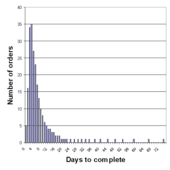 Figure 5: A skewed distribution
Given the Z-test's problems with non-normal data, and the fact that the permutation test is unaffected by different distributions, it is possible that the permutation test will be more accurate, and thus would be the preferred test. Theoretically, one should expect that the permutation test would calculate alphas that diverge from Z-test-produced alphas increasingly as sample sizes decrease - the smaller the sample, the larger the discrepancy. On the other hand, as sample sizes increase, the alphas from the two methods should converge toward equality for large samples. Unfortunately, the few data examples we have available to us do not show this expected relationship. 87 The examples show the expected divergence for small samples, but not the expected convergence for larger samples, contrary to the theoretical expectation that the results should be the same for large sample sizes.88 These results raise doubts that the record before us is sufficiently developed to allow us to confidently select the permutation test as a superior test. Either the permutation test is treating data differently than we would expect, or a sample size of 30, or even 131, is still too small to expect sample mean distribution normality for these performance measures. We note that the permutation test is relatively insensitive to outliers89 compared to the Z-test. This insensitivity occurs because in the final step, the permutation test treats the data as ranked data where an extreme score's value does not influence the outcome.90 In contrast, extreme scores influence the Modified Z-test. 91
This result raises the question whether extreme scores would have insufficient influence in a permutation parity test, insofar as these extreme scores might be some of the most publicly noticeable indicators of discrimination. For example, an unusually long delay in obtaining a needed phone service can be especially troubling. Other issues regarding the selection of the Z-test or the permutation test are more fundamental. If it is more appropriate to view the ILEC and CLEC performance results as samples of a theoretically larger process, then the Z-test may be the more appropriate test. If it were more appropriate to view the ILEC and CLEC performance results as the whole population of production output, then the permutation test would be more appropriate. This underlying issue was raised in the ACR, but has not been resolved by the parties or the record in this proceeding. Until we can determine which test is the more appropriate treatment of the data, including underlying issues such as "production output" versus "larger process population sampling" and more specific issues regarding outlier treatment, we are not in a position to either order or approve use of the permutation test. The most important question of decision accuracy is not resolved. Additionally, we need to better understand what the appropriate sample sizes are for using the permutation test versus the Modified Z-test.
Consequently, we will order the Z-test used during the trial period for all average-based performance results. Most importantly, we will not order Pacific to implement a permutation test data analysis system since even the new lower cost estimates warrant a greater confidence than we currently have in the test's benefits relative to its costs. However, we recognize the permutation test's potential for being the more accurate test, especially if it is appropriate to view a CLEC result as a sample of a fixed production output result. As we believe it would be a mistake to leave unresolved the questions surrounding this test's potential, we direct the parties to conduct or fund a research inquiry to answer these questions. We prefer a collaborative research approach where all interested parties would collectively influence the research proposal, and thus would be more inclined to accept the results. But in the interim, the Z-test is the most developed and accepted alternative to permutation testing. We shall order that the Modified Z-test be used for average-based parity performance measures. We discuss further the problem of small samples in a following section.
Percentage-based measures
Modified Z-tests
While the parties have proposed Modified Z-test variants for percentage-based measures, and those variants are being used in New York and Texas, these measures present new difficulties for Modified Z-test application. For example, the test requires an ILEC variance. When there is perfect ILEC performance, the Modified Z-test statistic is not calculable.92 Pacific proposed a modification to the Modified Z-test for percentages based on the CLEC variance. The CLECs and Verizon CA proposed use of permutation tests, or more specifically, exact tests, which do not require calculation of ILEC variance.
Exact tests
Exact tests are called "exact" because if used consistent with necessary assumptions they calculate the exact probabilities of frequency (counted, rate, proportion) data.93 They represent a special case of permutation testing. The advantage for our statistical model is two-fold: (1) calculations are made directly from the raw data, and (2) exact tests have the potential to produce more accurate results for small samples. In the case of the percentage-based performance results data, the Fisher's Exact test is appropriate.94
The Fisher's Exact test calculates the probability of an obtained or worse result when the data conform to a two-row by two-column table. Such is the case in the analysis of percentage-based measures where, for example, the first row represents CLEC percentages with the number of "missed dates" for orders in the first column and the actual number of "met dates" in the second column. The second row similarly represents the ILEC data, creating a two-row by two-column data table, or a "2 x 2" table. Given such a table, there is a limited number of possible unique combinations, or permutations, of entries in each of the table's four "cells." The Fisher Exact test determines the probability of each individual combination that is as extreme or worse than the obtained combination being tested. The sum of these probabilities is the probability that the obtained result could occur if the results are only due to random variation.
This probability is "alpha," the probability of a Type I error. Unlike for average-based permutation applications, outliers cannot affect the result, as the data consist only of "cell counts." Additionally, unlike for average-based permutation applications, the results from the percentage-based Modified Z-test and the results from the Fisher's Exact test converge towards equality as theoretically expected.95 Additionally, the FCC has approved an application that uses the Fisher's Exact test for percentage-based measures.96 We shall order that the Fisher's Exact test be used for all percentage-based parity tests.97 The evidence before us indicates that it provides accurate decision error probabilities, is consistent with theoretical assumptions, solves the Z-test application problems, and generates no objections from the parties.
Rate-based measures
The problem, and our solution, for rate-based performance result analysis is similar to the case of percentage-based performance measures. In this case, a binomial exact test is applied to rate data because the Fisher's Exact test's assumptions are not met. Specifically, the Fisher's Exact test is not appropriate where the row totals are not fixed, or where an entity being observed can contribute more than one cell entry. In the case of percentage-based measures, the Fisher's Exact test is warranted because the row totals are always 100 percent, equal to the total number of CLEC or ILEC orders, and every order only creates one cell entry. In contrast, row totals for rates vary directly with the performance result. For example, the most common rate measure is service "troubles." The rate is typically taken as the rate of troubles per number of lines. This figure can theoretically vary from zero to a number greater than the number of lines because it is possible to have more than one trouble per line. Consequently the row totals are not fixed. However, in this case, assuming the parameters for a Poisson distribution, a binomial exact test can be applied to calculate the probabilities of rate performance results.98
Additionally, like the percentage-based Fisher's Exact test applications, and unlike for average-based permutation applications, the results from the rate-based Modified Z-test and the results from the binomial exact test converge towards equality as theoretically expected.99 Verizon CA, the CLECs, and ORA agree to the appropriateness of the binomial test100 and Pacific does not object. We shall order that the binomial exact test be used for all rate-based tests as the evidence before us indicates that it provides accurate decision error probabilities, is consistent with theoretical exceptions, solves the Z-test application problems, is preferred by most parties, and generates no objections from any party.
Confidence levels
Alpha levels
The specific fixed alpha levels that have been recommended in this proceeding are 0.15, 0.10, and 0.05 alphas, which correspond to the 85%, 90%, and 95% confidence levels, respectively. The 90% confidence level suggested in the ACR is no party's favored level. The ILECs, Pacific and Verizon CA, prefer a 95% level to minimize the possibility of payments made due to sampling error when there are no real differences. The CLECs and ORA prefer an 85% confidence level to minimize the possibility that the ILECs escape payments when there are real differences, but those differences are masked by sampling error.101 Each side wishes to protect against the negative effect of random variation. But since there are two possible effects of random variation, and as one is minimized the other is maximized, the two sides differ in the preferred confidence level.
Pacific and Verizon CA assert that the 95% level should be used since it is an accepted convention. We disagree. While we understand that it is a convention is some contexts, it is important to understand those contexts to see if they generalize to the present case. They do not. Academic texts that address the use of the 95% level, and that go beyond simply noting its common use as a convention, are clear in pointing out its arbitrariness in applied decision settings:
The widespread convention of choosing levels of 0.05 or 0.01 irrespective of the context of the analysis has neither a scientific nor a logical basis. The choice of level is a question of personal judgment in the Fisherian approach and one of considering type I and II errors in the Neyman-Pearson approach. Since for a given sample size decreasing one error probability increases the other..., it is possible to argue for a relative balance. In particular, if at _ = 0.05 the power is very low, one might seriously consider increasing _ and so increasing the power.102
In our opinion, there is no "right" or "wrong" level here - the decision must be made in full consideration of parameters inherent in the problem itself. It is doubtful that setting a priori levels of .05, .01, or what have you settles the matter.103
No absolute standard can be set up for determining the appropriate level of significance and power that a test should have. The level of significance used in making statistical tests should be gauged in part by the power of practically important alternative hypotheses at varying levels of significance. If experiments were conducted in the best of all possible worlds, the design of the experiment would provide adequate power for any predetermined level of significance that the experimenter were to set. However, experiments are conducted under the conditions that exist within the world in which one lives. What is needed to attain the demands of the well-designed experiment may not be realized. The experimenter must be satisfied with the best design feasible within the restrictions imposed by the working conditions. The frequent use of the .05 and .01 levels of significance is a matter of a convention having little scientific or logical basis. When the power of tests is likely to be low under these levels of significance, and when type 1 and type 2 errors are of approximately equal importance, the .30 and .20 levels of significance may be more appropriate than the .05 and .01 levels. (p. 14, emphasis added.)104
In principle, if it is very costly to make an error of Type II by overlooking a true departure from [the null hypothesis] but not very costly to make a Type I error by rejecting [the null hypothesis] falsely, one could (and perhaps should) make the test more powerful by setting the value of [alpha] at .10, .20, or more. This ordinarily is not done in social or behavioral science research, however. There are at least two reasons why [alpha] seldom is taken to be greater than .05: In the first place. . . in such research the problem of relative losses incurred by making the two kinds of errors is seldom addressed; hence conventions about the size of [alpha] are adopted and [beta] usually is ignored. The other important reason is that given some fixed [alpha], the power of the test can be increased either by increasing sample size or by reducing the standard error of the test statistic in some other way, such as reducing variability through experimental controls. (P. 290.)105
These four quotes point out the dilemma in our applied problem. Unlike in scientific applications where the parameters of an experiment are easily manipulated, we have neither the luxury nor the discretion to change the sample size, the effect size, or the sampling error. Consequently, the Commission must chose an alpha level without regard for conventions developed in qualitatively different contexts.106
Additionally, while the authors of the last two quotes appear to differ in their recommendations regarding the relative consequences of Type I versus Type II error, these differences should be viewed in terms of different assumptions regarding the freedom to change sample sizes, error terms, and the strength of experimental treatments, among other parameters. Academic treatises directly addressing these relative consequences have developed formulas that balance the net consequences of any resultant error by establishing loss functions. 107
For example, while different alpha, and thus beta, levels are appropriate depending on the ratio of the costs of the consequences of both types of errors, when the error consequences are deemed to be equal, losses are minimized when alpha and beta are set to be equal.108 We have not determined a specific ratio for the relative consequences of failing to identify competition barriers when they exist versus monetary payments made when they should not be made. However, at this point we can only assume from the purpose of the Act and the regulatory policy mandating competition, that the consequences of not identifying barriers is at least equal to any misappropriated payments. As a consequence, our goal will be to choose an alpha level that serves to balance with a beta level.109 In doing so we are not addressing risk. The question of relative risk is more appropriately addressed in the proceeding's next phase, which will establish the "consequences" for the performance decisions made in the present phase. Balancing alpha and beta to be equal only ensures that the most accurate decision is made, not what the consequences of those decisions will be.
We note that the FCC encourages such a balance.110 We also note that the NYPSC has adopted as low as an 80% confidence level in certain circumstances, possibly to achieve a better balance. While we have discussed a 90% confidence level as a compromise to facilitate negotiation progress, we are unwilling to permanently select such a fixed level based solely on the midpoint between two negotiating positions.
Pacific argues against the 90% confidence level stating, "There is no forum of which we are aware that supports the use of a 10% error rate." However, we find it notable that the BANY remedies plan uses a 21% error rate (79% confidence level) for conditional failure identifications and a 10% error rate for final determinations.111 We also note that one of the statistical texts frequently cited in the FCC's BANY 271 approval states, "The value of alpha chosen is usually between 0.01 and 0.1, the most common value being 0.05."112
Although Verizon CA presents an academic cite as justification for its preference for a 95% level (.05 alpha), we find that that cite refers only to less formal "rough conventions" and does not refer to any context or consequences of the two different types of error.113 Additionally, Verizon CA quotes an affidavit in a FCC proceeding citing an AT&T statistician's support for the 95% level. We also do not find that quote necessarily applicable to the problem of balancing the two errors. In that quote, Dr. Mallows states that a 95% level would control Type I error "while making the probability of Type II errors small for violations that are of substantial size."
The Commission cannot base its decision on such a statement when the statement context is not clear. At the time Dr. Mallows made the statement, over two years ago, it may not have been apparent how small the sample sizes were going to be, and thus he may have been referring only to results obtained from fairly large samples. We are concerned that even substantial Type II errors may not be identified with a 0.05 alpha level for small-to-moderate samples. Additionally, Dr. Mallow's statement implied that the statistical test, through its significance level, was used to determine magnitude as well as statistical significance. We cannot know how Dr. Mallows' statement applies to our context without knowing what he meant by the term "substantial." But more importantly, our approach is different. We will address the magnitude issue separately below after the error problem has been addressed.
A deciding factor for us is the potential consequences of the two types of error to our overall performance remedies plan. Given the potential for us to err on one side where we might favor either alpha levels or beta levels to the detriment of the other, the correctability of any such imbalance that might result is an important consideration. On one hand, if we set alpha too large and as a result make Type I errors, we can make up for these errors in the incentive-amount methodology phase of this proceeding. For example, we could adjust the incentive amount to the actual Type I error calculated for each performance result. Specifically, presented for illustration purposes only, we could levy an incentive payment for a result with a Type I probability of .95 at 95% of a pre-determined amount, but levy a payment with an alpha probability of .85 at 85% of the same amount.114 In contrast, once we have made a Type II error, no correction is possible since parity would have been concluded. In this case the measurement would not make it to the incentive payment phase, and thus would not be correctable.
We note that the NYPSC addressed this issue by selecting three alpha levels: a 0.05 alpha level for immediate non-parity identification, approximately a 0.20 alpha level for conditional parity identifications depending on subsequent months' results, and a 0.10 alpha level for final disposition of conditional identifications.115 The parties have variously proposed the 0.05 or the 0.15 alpha levels, and the ACR recommended a 0.10 level for the purposes of development, inquiry and compromise. However, we are not comfortable selecting alpha levels without discussing and assessing beta and its converse, test power.
Test power
Unfortunately, the record is relatively silent on the actual beta values that various critical alpha levels might produce. The only estimates in the record are that in early tests, AT&T estimated betas to range as high as 0.21 when critical alpha levels were set to 0.05.116 A beta value of 0.21 corresponds to a test power of 0.79, or 79%. AT&T also estimated that if alpha was set to 0.15, then betas would average a similar level - an average test power of 85% when the average Type I confidence level is 85%. Yet it is unclear if the results from the earlier tests are comparable to the performance results in California. To remedy this lack of critical information, we shall direct the ILECs to calculate both alpha and beta values whenever a statistical test is applied.
Staff has performed some preliminary estimates of beta values using four different alpha levels.117 The results are discouraging about the ability of our model to perform its most fundamental task, to detect competition barriers. For example, with a 0.10 critical alpha level, and selecting a 50 percent difference to establish alternate hypotheses, beta values average 0.63 with a median of 0.79.118 While the selection of a 0.10 critical alpha threshold ensures that 100 percent of the performance results are subject to a 10 percent maximum Type I error, it only provides that 16 percent of the results are subject to a 10 percent maximum Type II error.119
Additionally, the parties have not recommended any minimum test power, or its respective error, beta. Since beta is determined by the other elements, the degree of test power ends up being that which results from the other elements. The record is relatively silent on the appropriate test power or beta error level. While unfortunate, this state of affairs is understandable since at the outset alpha can be set, but beta can only be determined upon obtaining the measured performance results. Beta will thus vary for every performance result. For every obtained result, however, it is possible to balance alpha and beta if we can safely make assumptions about two components of the analysis: (1) the relative consequences for each type of error, and (2) the specification of the alternative hypothesis.
As a general policy statement, it is reasonable to assume that a Type II error is at least as important as a Type I error, as discussed earlier. Apparent discrepancies can be adjusted in the incentive payment phase. However, specification of an alternative hypothesis is more difficult. The alternative hypothesis is the hypothesis that barriers exist - that ILEC service to its own customers is actually worse than to CLEC customers beyond that which could be explained by sampling error. We are aware of three ways to specify the alternative hypotheses. First, the critical value for the alternative hypothesis could be set to equal the critical alpha level value. This would not be much help because the beta error level would always be 50%.
Second, the actual result could be selected as the alternative hypothesis. It would be reasonable to assume that an actual result was the best estimate of the actual underlying process, and as such best represents the alternative hypothesis. A statistical test could then estimate the respective Type I and II errors of this result being a "true" mean, not identified due to sampling error. In this case, the balanced alpha and beta level could easily be determined.120 It is unclear at this point, though, what the effects of this balancing would be since for very small differences, both beta and alpha might be very large, whereas for big differences, both might be small. If this happens, we would still have to set some alpha/beta thresholds, and/or set some "material" difference thresholds.
Third, the critical alternative hypothesis value could be determined by identifying a performance result or level where ILEC and CLEC service differences become "meaningful." Verizon CA has proposed such performance levels, called "deltas," as a solution to a different problem in this proceeding.121 However, the record contains no information on what those deltas would be, as no party has submitted any proposal containing a comprehensive set of specific deltas.
A fixed alpha is not an adequate long-term solution. As the CLECs have asserted and as staff's data analysis has shown, test power is very low for the small samples that represent the majority of the performance measure results. On the other hand, the ILECs have asserted, and staff's data analysis confirms, that fixed alphas that provide better test power for small samples result in unnecessarily high test power for large samples. This unnecessarily high test-power can easily result in meaningless differences being found statistically significant.122 We believe that the problems of insufficient test power for small samples (large beta) and "too much" test power for large samples can be better resolved through even approximate alpha/beta balancing techniques. We direct the parties to develop and implement an alpha/beta balancing procedure for our model. However, to give sufficient time for its development without delaying Pacific's 271 application, we shall adopt a fixed alpha solely for the interim, and shall order that the balancing components to the model be added by the end of the trial period unless the parties reach agreement and move to implement the components sooner.
Fixed alpha
We conclude for the reasons cited above that a fixed alpha critical value should only be used as an interim decision-criterion solution. Setting alpha to remedy one problem only makes another. We select a larger alpha level, 0.10, instead of the 0.05 level to enhance decision accuracy and to avoid uncorrectable decision-making errors while still being able to address correctable errors in the next phase of this proceeding. We select a smaller alpha level than 0.15 because we are concerned about the effect on large-sample results. We have selected the 90% confidence level (0.10 alpha, or 10% significance level) to control the Type I error and to reduce the Type II error to more acceptable levels for the preponderance of the performance results. That is, we choose to be at least 90% confident that any barriers we identify represent real differences, not differences due to sampling error (random variation), while increasing the average confidence level (power) for detection of actual differences from 30% for the 0.05 alpha to 37% for the 0.10 alpha.123
Additionally, because of the low power of these tests, we also adopt the 80% confidence level (0.20 alpha) for conditional failure identifications. This threshold is used in the BANY performance remedies plan for conditional identifications where results at 0.20 alpha or less were deemed failures if they occurred in two months of a three-month period.124 We will not dictate the additional specifications for such conditional identifications, but instead direct parties to set forth those specifications in the next phase. Among other possibilities, our plan could have additional criteria such as (1) successive failures such as in the BANY plan, (2) alpha and beta balance at values less than 0.25, or (3) for CLEC-specific performance assessment, industry aggregate performance out of parity. Noting that if a 80% confidence level (0.20 alpha) was used as the overall fixed threshold instead of the 90% level (0.10 alpha), average power would increase from 37% to 48%,125 we wish to take advantage of this increased power at least on a conditional basis.
Material differences
None of the parties have specified the minimum differences (effect size) between the ILEC and CLEC performance results that would identify a competition barrier. Two parties have raised the issue. AT&T has somewhat tangentially raised the issue in its discussion of test power126. To calculate test power, an alternative hypothesis must be specified as discussed supra. AT&T estimated test power across an array of different performance results after subject matter experts made judgments creating competition-affecting performance thresholds.127 Verizon CA currently proposes utilizing "deltas" which embody virtually the same concept, albeit for different purposes. Whereas AT&T created thresholds to investigate insufficient test power, Verizon CA proposes to create these conceptually identical thresholds to investigate "too much" test power.128 We find that both efforts to establish "material" thresholds have merit. First, as we have described above, test power is a primary decision-accuracy concern for this remedies plan. The best way to calculate test power is to specify a meaningful alternative hypothesis, and the most meaningful alternative hypothesis is one that embodies the core performance remedies plan goal, barriers to competition. Second, it would be contrary to the same decision accuracy policy goals to impose incentive payments when an ILEC is providing virtually the same service to a CLEC that it is providing to itself with no negative impact on competition. Recent academic discussions have pointed out that in the case of large samples, statistical results right at an alpha level of 0.05, for example, can provide evidence for the null hypothesis, rather than against it as designed:
Results indicate that for point null hypotheses, a statement of [statistical significance at alpha] does not have a straightforward, evidential interpretation. It is demonstrated, that for larger samples particularly, that a report merely that data are [statistically significant at alpha] has no objective meaning, and under some conditions should be interpreted not as evidence against the null hypothesis, as is usually supposed, but as strong evidence in its favor.129
For very large samples, significant differences at or close to the .05 threshold might be so negligible as to be perceptually the same to a CLEC customer as would be the "statistically significantly different" ILEC service, and as a consequence actually be evidence of parity, not discrimination. Statisticians seem to agree that statistical significance is different from substantial significance.130
We find that the "material difference" standard has merit and the potential to improve the decision model we specify. However, we are concerned that the task to construct a set of difference thresholds is difficult, and yet to be accomplished in any collaborative forum. We encourage the parties to complete this task as part of the alpha/beta balancing task we order today. However, since other ways to specify an alternative hypothesis may be easier to accomplish, yet sufficient to enhance decision accuracy, we will not order the material differences be defined for every measure. Other methods for balancing alpha and beta errors may resolve the material difference versus statistical difference problem and we choose to allow the parties the discretion to collaboratively determine the best solution before we order our own solution.
Optimal alpha and beta levels
The parties have variously discussed "equal risk," "equal error," and "balancing alpha and beta." "Equal risk" refers to a situation where the expected consequences of the performance remedies plan are the same for an ILEC as for the CLECs. The concept of equal risk is beyond the scope of our decision model as it necessarily requires incentive payment specification which we will not consider until the next phase of this proceeding. "Equal error" and "balancing alpha and beta" refer to a situation where the two possible decision-making error probabilities are the same. We endorse the concept not only because it meets our fairness principle, but also because it maximizes decision accuracy.
Overall decision error is minimized when alpha and beta are balanced.131 But most importantly, if we are to create a "level playing field," we must be fair in our acceptance of decision error. The data shows that a fixed alpha level of 0.10 can only be suitable for an interim implementation because it favors reducing the error that only the ILECs wish to reduce. There would be no level playing field if we tolerated no more than 10 percent error harmful to the ILECs, yet tolerated 40 to 60 percent error harmful to the CLECs. We only take the 10 percent alpha level as an interim compromise necessary for progress. Additionally, maximizing decision accuracy by equating possible errors is an appropriate first step to optimizing equal risk, and does not necessarily interfere with the consequence-setting function of the next phase of this proceeding. We direct the parties to work collaboratively to develop and implement an alpha/beta balancing decision component for our decision model by the end of the trial period. If the parties are unable to agree on such a model component at that time, we shall direct parties to submit their individual models for our review and decision.132
Minimum sample size
Minimum sample size requirements vary depending upon the type of statistical test used. For example, as discussed above, exact tests are not dependent on inferences about the underlying distribution, therefore the accuracy of calculated alphas is relatively unaffected by sample size. Therefore we find it necessary to discuss sample size issues individually for each type of measure.
Average-based measures
Sample size requirements for average-based measures are the most difficult to resolve. On one hand, the CLECs have pointed out the importance of separately assessing performance for even the smallest CLEC with the least activity since these CLECs depend more on each order or service than do the larger CLECs. Harmful ILEC performance in small new or innovative market niches, or harmful ILEC performance to smaller CLECs could be masked by larger market samples or larger CLEC samples when the results for CLECs are combined ("aggregated"). If so, then the smaller markets and the smaller CLECs would not be provided the protection that this performance remedies plan is supposed to provide. Such small CLECs and markets effectively would be unprotected by competitive market reforms, and thus might fail.
Consequently, the CLECs have urged sample sizes small enough to protect these markets. We agree with this principle, and thus, one goal of our plan is to assess each CLEC's performance results for each submeasure. On the other hand, as sample sizes become small, Central Limit Theorem states that the normality desired for Z-tests can no longer be assumed. The accuracy of the error estimates, alpha and beta, becomes suspect with the smaller samples. So we are faced with the potential dilemma of having to choose between achieving greater decision accuracy or protecting an important sector of the market. The parties predictably were not able to agree on a solution to this dilemma. Proposals ranged from a sample size minimum of 1 to a minimum of 50 or more.
The issue is relatively simple for the ILECs. They are concerned that small samples could produce inaccurate error estimation, which could inappropriately subject them to payments even when their processes are non-discriminatory. However, since the ILECs are more concerned with alpha levels, unlike beta levels, alpha levels can be held constant regardless of the size of the sample. So even though there may be an issue of accurate alpha estimation, there is still some adjustment as sample sizes decrease - alpha error is held constant. Additionally, with alpha error held constant and as sample size decreases, test power decreases, thus reducing the ILEC's potential liability under any performance remedy payment plan. On the other hand, the ILECs may be concerned that smaller samples generate greater incentive payment exposure by the consequent that there are more performance tests. However, this concern is best addressed in the incentive payment phase where it can be accommodated if warranted. The ILECs also prefer aggregation of all results, since in their view, the total result is the best indicator of the parity of the process.133 As a compromise, the ILECs offered to use sample sizes from 5 to 20, and they have offered to aggregate results in order to achieve these minimum numbers. With a few exceptions, the ILECs wish to exclude, from the performance remedies plan, data that does not meet these sample minimums.134 For example, samples that contain four or less observations after aggregation rules have been applied would be discarded unless they are a designated "rare submeasure" that should be analyzed regardless of sample size.
The issues for the CLECs are more complicated. On one hand, since increasing the sample size increases test power as the significance level is held constant, the CLECs would seem to prefer larger samples. Smaller samples often have negligible test power. However, on the other hand, the CLECs prefer no aggregation of results since the actual service each company receives is critical to them. Each company is directly affected by the service it receives from the ILEC independently of the service that other CLECs receive. Consequently, the CLECs have urged inclusion of sample sizes small enough to protect these markets. Second, the CLECs urge that all data be analyzed regardless of sample size. They do not want any data discarded from the performance remedies plan. It is unacceptable to the CLECs to ignore poor performance to a small emerging CLEC, simply because of a minimum sample size rule. However, like the ILECs, the CLECs agreed to a compromise position, accepting some aggregation rules, but firmly rejecting exclusion of any performance results because of insufficient sample size.135
Assisted by Pacific's technical expert, staff examined how one possible compromise set of aggregation rules would function.136 In summary, the rules were as follows: (1) Samples of 10 or more would be separately analyzed; (2) All samples of less than 10 would be aggregated for a collective analysis if they achieved at least a sample size of 5; (3) Where a minimum of 5 was not achieved, the remaining samples would be aggregated for analysis with all other CLECs for the submeasure; and (4) Where the industry aggregate did not achieve a minimum of 5 the data would be discarded.137 Using these rules, for the most recent month presented, March 2000, 57 percent of the performance results could be analyzed without aggregation, 39 percent could be aggregated with other small sample results, 1.3 percent had to be aggregated with the rest of the industry, and 2.4 percent of the results had to be discarded.138 While not having an opportunity to comment on this, the CLECs can be anticipated to object to these rules insofar as they require that 43 percent of the results be aggregated or discarded and that 3.7 percent (127) be either aggregated with the whole industry, possibly rendering their results masked by a much larger sample, or be discarded.139
Staff found several unresolved problems with the proposed compromise aggregation rules. First, in some cases, even with very low test power for a reasonable alternative hypothesis,140 the performance results to a small CLEC were highly statistically significant with an extremely low Type I error, or alpha. However, the aggregation rules caused this result to be combined with and masked by results for large CLECs. Second, in other cases, where several small CLECs experienced better or nearly equal ILEC performance, exceptionally poor performance to one CLEC caused the aggregate performance to be identified as a failure. Such an outcome could trigger payments to each of the CLECs, thus spuriously expanding the ILEC's liability.
Third, the aggregation rules caused some unnecessary aggregation. For some submeasures where only one CLEC did not have the minimum of five or ten results, its results were aggregated across the entire CLEC industry, which often had more than a thousand individual performance results. This would occur even though aggregating with only the smallest CLEC result over five or ten would have provided a sufficient sample size. With the proposed rules the small CLEC result was unnecessarily completely masked by the very large CLEC samples.
Fourth, in cases where there are multiple results for the same CLECs it is not clear which result would be used. For example, when a small CLEC's results are aggregated with larger CLECs' sample sizes that are small, but which are big enough to be analyzed on their own, two different conclusions could be reached. When the larger individual sample results all pass and when the combination of these results do not pass, the individual larger samples will be deemed to have passed individually but not in the aggregate. This result poses a dilemma in that on one hand the aggregate may be the better indicator of the larger process if one assumes a "process model," but on the other hand, assuming a "service model," only the smallest CLEC suffered harm. Each assumption suggests a different remedy.
We believe that it is important to examine performance at the smaller market and smaller CLEC levels. This market arena may be critical for entry and innovation, which in turn are critical to a healthy competitive telecommunications infrastructure. However, given the unresolved issues for sample size and aggregation rules, and the fact that the rules for incentive payments are integrated with the aggregation rules, we are reluctant to permanently order any minimum sample sizes because any such minimums would require some data be discarded. Before finishing this discussion, we examine proposals that might not require sample size minimums.
Permutation testing has been proposed as a solution to the Z-test's small sample normality assumption violations. We prefer use of the permutation test rather than the complicated, and somewhat confusing, data elimination and aggregation rules. However, as we discussed earlier, the record is not sufficiently complete for us to be confident that permutation testing is free of other problems. In New York, while permutation testing is being developed, the New York Public Service Commission has ordered t-tests used for small samples as an interim solution for the Z-test small sample problem.141
Statistical texts indicate that the t-distribution is more appropriate for tests between two sample means, especially for small samples.142 Use of a t-distribution "look-up" table could alleviate some ILEC concerns regarding possible alpha estimation inaccuracy for small samples. For example, with the current fixed critical-Z decision rules, a Modified Z-test statistic of 1.8 would identify a failure at all parties' favored alpha levels since it exceeds the most conservative proposed critical value of 1.645. This result would be the same for all sample sizes including a sample size of one. However, the ILEC's concerns regarding alpha accuracy increase as the sample size decreases. Using the t-distribution table would adjust for decreasing sample size. For example, for an ILEC sample size of two (df = 1), a critical value of 3.078 must be exceeded for the 0.10 alpha level.
Our example of a Z-statistic of 1.8 would not be significant unless the result sample size was at least four, since the critical t for a sample of 3 (df = 2) is 1.886 and the critical t for a sample of 4 (df = 3) is 1.638.143 Consistent with the academic justification of the Modified Z-test, we shall order the test statistic compared to the t-distribution. In this regard, we will refer to the Modified Z-test hereinafter as the Modified t-statistic, also consistent with its academic reference.144
Unfortunately however, this adjustment affects only the relatively infrequent small ILEC samples and not the preponderance of small CLEC samples.145 Additionally, other questions still remain regarding the accuracy of alpha estimation even with more conservative t-distribution tables. Even though the t-distribution is a remedy for small samples, its appropriate use still assumes the population is normally distributed, especially for one-tailed tests.146
We find that the controversies over the appropriate minimum sample size involve several unresolved elements of our decision model: alpha estimation accuracy, permutation or Modified Z-test use, aggregation rules, data exclusion rules, and incentive payment rules. For the reasons that there are several possible solutions to the minimum sample size problem, the resolution of any one of these problems may resolve the others, and the ultimate solution may necessarily involve decisions about incentive payment rules, we are reluctant to order a permanent minimum sample size. We are concerned that without further information, research, and calibration information, we would be essentially deciding "in the dark." While we prefer not to delay specifying final model components, in this case the complexity of the problem and the potential for a better solution warrants the delay. A better solution may be achieved during the calibration phase when parties can see how various rules, tests, and distributions work.147
However, we also are concerned that the parties may not either create or agree on a better solution to the small sample size problem. If this turns out to be the case, then we would in effect be ordering many applications of statistical analyses and decision rules for samples as small as one or two individual performance results. We find that we need to set some minimal rules that, in the case that parties are unable to agree on better solutions, will reduce dependence on such very small samples. We shall order the following rules as an interim solution as a "floor" for sample sizes. These rules are designed to avoid discarding any data, and to increase sample sizes for the very smallest samples with minimal impact on the actual results. These rules are also designed to be easily understood with the results easily reproduced. We find that the previously proposed rules are complicated and fall short of our goal of simplicity.
The following rules shall be used for average-based parity performance measures:148
(1) For each submeasure, all samples with one to four cases will be aggregated with each other.
(2) Statistical analyses and decision rules will be applied to determine performance subject to the performance remedies plan for all samples after the aggregation in step (1), regardless of sample size. For example, if samples with as few as one case remain after the aggregation, statistical analysis and decision rules will be applied to determine performance subject to the performance remedies plan to these samples, just as they are for larger samples.
These small sample aggregation rules minimize most of the problems described above for Pacific's proposed plan. (See Appendix I.) We do not presuppose how payments will be triggered or allocated under these aggregation rules. The issues will be addressed in the upcoming incentives phase. For example, the parties can decide whether any CLEC whose results are aggregated into a failing aggregate, yet whose individual results are better than the ILEC parity standard, should receive incentive payments. In this case, an "underlying process" model might suggest that this CLEC receive payment because the process was flawed and the incentive was necessary to motivate process improvement. On the other hand, a "service" model might suggest that this CLEC not receive payment since it suffered no competitive harm. Parties will have an opportunity to propose and discuss different treatments of the outcomes from different sample sizes.
Percentage and rate-based measures
The fundamental problem with small sample sizes for average-based parity measures is that they fail to satisfy the normality assumptions for the Modified Z-test. In contrast, percentage and rate-based measures are assessed using exact tests, which do not depend on inferences or assumptions about underlying distributions. Consequently, with these tests there is less concern with the accuracy of the alpha and beta calculations for small samples. We find no other compelling reason to aggregate or discard data, and thus, we direct that all percentage and rate-based data at the submeasure level for each CLEC be analyzed for parity regardless of sample size.149
Data transformations
Pacific proposes a Modified Z-test enhancement to address the data non-normality problem for average-based measures. Pacific asserts that for lognormal data distributions, transforming raw scores to their natural logs can bring the distribution close to normality, and thus satisfy the essential assumption for using a Z-test.150 The CLECs agree to such transformations.151 Verizon CA and ORA accept the transformation proposal in concept, but both are reluctant to use it without further research. We agree with Verizon CA and ORA so far as the record is not clear how such transformations might affect decision accuracy. However, academic sources provide guidance. For example, one text states,
"The logarithmic transformation is particularly effective in normalizing distributions which have positive skewness. Such distributions occur... when the criterion is in terms of a time scale, i.e., number of seconds required to complete a task."152
This is precisely the type of measure on which the average-based parity performance measurement is based.153 So from a theoretical perspective, the log transformation is appropriate and reasonable. Additionally, staff has performed analyses on several qualitatively different performance results. From these analyses, staff has concluded that a log transformation (1) brings the distributions much closer to normality, and (2) provides a reasonable interpretation of skewed data. Staff's analyses of several ILEC and CLEC distributions are included as Appendix J. These analyses show the improvement when log transformations are used. In addition, they demonstrate that even in cases where the log transformation dramatically changes results from the non-transformed data, the transformed results are reasonable and appropriate treatments of the performance data.
Transformations also change the effect of outliers. For example, when an outlier exerts influence on the average result in small samples, transformations can change even the direction of the performance result from worse performance to better performance.154 In another case, we note that the probabilities even for large samples where there should not be large differences change dramatically when scores are transformed.155 While the data sets we reference may be unique examples, they raise questions that we should resolve, but are not in a position to entirely do so from the record in this proceeding to date. For the above reasons, we decline to order transformations of the data on a permanent basis unless the record is adequately developed in subsequent phases of this proceeding. Additionally, our preference is that more exact tests be used, if appropriate, which solve the small sample normality problems without transformations.
However, since we must still use the Modified Z-test, and since we must apply it to samples where normality can not be assumed, then we find that the log transformation is reasonable and appropriate, and is at least as an interim solution is necessary for application of the test to small to moderately large samples. We also find that the transformation improves normality for large samples.156 Therefore, we shall order that log transformations be utilized for all average-based performance measures as specified in staff's analysis in Appendix J.
This still leaves us with the issue of the meaning of outliers. If the impact of outliers should be minimized in our performance assessment, then the log transformations accomplish this and nothing further needs our attention. However, if outliers are meaningful in their own right, then we need to address the issue. As stated above, it is plausible that an outlier can have a disproportionate affect on competition when in the CLEC sample. Very long provisioning times could gain notoriety that could harm the reputation of a CLEC. On the other hand, outliers in the ILEC results could raise the mean and mask the fact that the ILEC is providing predominately superior service to its own customers. We believe this issue should be discussed in the incentives phase of this proceeding, and we will be open to proposals for a separate treatment of outliers in their own right. But even if parties do not propose a separate treatment of outliers or agree on their meaning, we are convinced that the log transformations provide a more appropriate Modified Z-test application. If further deliberations and negotiations of the parties do not result in adequate development of permutation testing or outlier treatment, at this point we accept the fact that log transformations may become the permanent solution.
Benchmark issues
In contrast to the parity standard for CLEC performance results with ILEC retail analogues, where there is no retail analogue, the standard is performance that allows a "meaningful opportunity to compete." In the performance measurement phase of this proceeding, the parties agreed to establish "benchmarks" which specify such performance levels.157 Since there is no measure of an ILEC's internal performance (i.e., no retail analogue), there is no ILEC variability on which to base an expected performance parity standard. Consequently, parties negotiated measures with thresholds that would allow CLEC service access judged to allow a meaningful opportunity to compete.
The parties discussed two contentious issues regarding benchmarks. The parties discussed alleged problems of small sample sizes causing falsely missed benchmarks and random variation causing falsely missed benchmarks. Pacific proposed using adjustment tables to remedy the sample size issue and statistical testing to remedy the random variation issue.
Benchmark adjustment tables
Pacific contends that performance measures for small samples present problems in that some benchmarks would not be met even though an ILEC provided adequate service. For example, if a benchmark established that 90 percent of orders for a particular service must be complete within a certain timeframe, then for every 100 orders there could be 10 missed timeframes without failing the benchmark. Pacific points out that for small samples, one failure could drop performance below the 90 percent level. For example, if only five orders were made per CLEC, then across 20 CLECs (100 orders) there could be 10 missed timeframes (90 percent on time) and for this aggregate performance a "meaningful opportunity to compete" could be assumed by original agreement of the parties. However, at least two and at most ten CLECs in this example would have missed the benchmark. That is, if ten CLECs missed one timeframe each (for a total of 10 missed timeframes), then they each would have performance measure results of 80 percent. At least two CLECs would have to fail the performance measures (5 failures each for the total of 10 missed timeframes) even though performance was right at the benchmark.
Recognizing this problem, the CLECs have agreed to allow adjustments to the benchmark outcomes, although not to the extent desired by Pacific. Noting that benchmarks were created under the federal definition of performance allowing a "meaningful opportunity to compete,"158 we are reluctant to allow less than the levels set by the benchmarks. To do so suggests less than a "meaningful opportunity to compete." However, in this case, because of the legitimacy of the small sample problem, and since the CLECs have agreed to some adjustments, we shall include an adjustment table in our decision model. Although the ILECs and the CLECs agree to use a benchmark adjustment table, they disagree on two aspects of such tables, sample sizes to which they will be applied and sample sizes from which they will be derived.
For the application of the adjustment tables to benchmarks results, the CLECs agree to the use of adjustment tables up to a performance result sample size of 30, and propose they be used down to a sample size of 1.159 The ILECs propose using the tables for performance result sample sizes up to 100, down to 10 with no aggregation, and down to five with the aggregation rules they proposed for parity measures as discussed above.160 The difference between the two proposals appears to be the type of problem they address. The CLEC table proposal appears to be addressing more closely the data "granularity" problem161 as we have described above, whereas the Pacific table proposal appears to go beyond data granularity and address broader statistical applications to benchmarks as we discuss below.
The ILECs and the CLECs also differ on the second issue, the adjustment table derivation sample size. The CLECs argue that since the table will be used on small samples, the tables should not be derived from larger samples. While they wish to limit the table's application to samples of 30, as a compromise they offer to base the table's derivation on a sample size of 100. Pacific wishes to derive the table from a sample size of 1000, but offers a derivation sample size of 400 as an alternative. Pacific states that a derivation sample size of 400 or 1000 is appropriate because the "implied performance" resulting from these derivation sample sizes is closer to the benchmark and is not unreasonably larger as would be the case with the CLEC's proposed derivation sample sizes.
While the CLECs' position is intuitively attractive in terms of the construction of the table, we appreciate Pacific's analysis because it assesses at least one net effect of the table. However, just as we are concerned with inferential statistical testing issues, we are concerned that other essential net effects have not been considered, namely the net effect that adjustment tables have in lowering the effective benchmark levels. For example, Pacific's adjustment table would allow performance to drop well below the nominal benchmarks without any failures being identified. Where the adjustment tables are applied, performance could average as low as 82 percent or lower across all performance results.162
Additionally, we are concerned that "one size fits all" application and derivation sample size specifications may not be appropriate. For example, we note that the smallest application sample size where a whole integer failure matches the nominal 90 percent benchmark limit is 10, yet the similar smallest sample size for the nominal 99 percent benchmark is 100. 163 We find it appropriate to set different application sample sizes for different benchmark percentage levels. In the same manner, we find that a fixed derivation sample size results in varying levels of implied performance relative to the benchmark limit. For example, a derivation sample size of 400 for the nominal 90 percent benchmark results in a 92.9 percent implied performance level, which is a 29 percent movement toward perfect performance.164 In contrast, the same derivation sample size of 400 applied to the nominal 99 percent benchmark results in a 99.68 implied performance level, which is a 68 percent movement toward perfect performance.165 We find that the appropriate application and derivation sample sizes vary with the benchmark level.
Inseparable from the problem of the granularity of the data affecting the implied performance is the affect that any adjustment will have on the established benchmarks. For example if one miss is allowed for a nominal 90 percent benchmark when applied to a sample size of five, then the benchmark percentage is effectively changed to 80 percent. Using the example of 20 CLECs with samples of five cases each as discussed above, all 20 CLECs can experience 80 percent performance without failures being identified. The overall performance for the total submeasure would be 10 percent below the nominal benchmark.
Staff has summarized the net changes to the nominal benchmarks in Appendix K. It is clear that when the adjustment tables are used, the benchmarks are substantially lowered. Recognizing these potential changes, we conclude that the implied performance level should address what is analogous to a Type I error without disproportionately increasing what is analogous to a Type II error. In other words, the implied performance level allowance should be higher from the nominal benchmark to a similar degree as the adjusted benchmark is effectively lowered from the nominal benchmark. With this balance in mind, we find that the application and derivation sample sizes recommended by staff in Appendix K, are more appropriate than the parties' proposals. Consequently we shall order the ILECs to use the small sample adjustment tables presented in Appendix K.
Benchmark statistical testing
Pacific and Verizon CA also favor complete statistical testing for all benchmarks. They assert that benchmarks are subject to the same random variation problems as are parity measures. However, Pacific only acknowledges the effect of random variation on alpha and only presents remedies for alpha. We are concerned that these adjustments increase beta, and since we are at least as concerned about effects on beta, we are reluctant to make the statistical adjustments recommended by Pacific. Additionally, we interpret benchmarks to be absolute performance limits that define a "meaningful opportunity to compete." Pacific argues that the benchmarks were created before statisticians were involved and before performance data was available, and thus the "negotiators relied on their experience in telephony and the needs of the CLECs to arrive at plausible benchmarks," and "did not fully appreciate. . . or consider. . the potential effects of random variation. . . ."166 Yet Pacific goes on to admit that benchmarks were set recognizing that "the process in question is not completely controllable." (Id.) Pacific's speculation about what was in the minds of the negotiators is contradictory and unpersuasive. We have no confidence in basing a new statistical overlay on such speculation, as we similarly have no confidence in rejecting telephony expertise for statistical expertise.
It is clear to us that the benchmarks already allow for random variation - no benchmark requires all services to be completed within a certain time period, and no benchmark sets a limit on the degree of any one service's outcome. For example, if the benchmark is 90% of orders completed within 4 days, and 92 percent of the actual orders were completed in 4 days or less, then Pacific is not held accountable for the random or even non-random variation of the remaining 8 percent. It would make no difference in the remedies plan whether these orders were completed within 5 or 100 days.
We are concerned that adding any additional tolerance margin to existing tolerance margins would allow two or three bites at the same apple. We prefer that if the benchmarks are not consistent with their definition of performance that will allow "a meaningful opportunity to compete," that they be adjusted directly, rather than add all the complexities and ambiguities that a new statistical overlay would create. With the inclusion of the adjustment tables we specify above, we shall order that benchmarks be treated as tolerance limits. This is an issue that may be re-examined in the incentive payment phase.
Benchmark modification
Closely related to the problems that the adjustment tables and statistical tables are intended to address is the benchmark levels themselves. One possible view is that instead of using adjustment tables that the benchmarks themselves be adjusted. However, since the adjustment depends on the sample size, different benchmarks would have to be set for different sample sizes. This would be virtually the same as using adjustment tables with the current benchmarks. Consequently, we will not order a review and revision of the benchmarks at this time.
Correlation analysis
All parties agree that performance measures that are correlated because they are redundant should be treated so that multiple payments are not made for the same failure. At the same time, parties recognize that a statistical correlation alone cannot distinguish between failure redundancy and multiple instances of independent discrimination. No party wishes to implement a self-executing statistical correlation component to reduce payment for discrimination. Since our immediate concern here is for the self-executing performance remedies plan, we do not order any statistical correlation component to our decision model at this time.
We also find that parties presented correlation analysis only as an abstract concept. No implementable plans were described or proposed. If any party wishes for us to consider a correlation plan we ask that they describe a plan down to the level of detail that will allow implementation. For example, it will be important to understand what data will be analyzed, what analyses will be employed, what decision criteria will be used, and what follow-up will be used to distinguish redundancy from multiple discrimination. The plans should provide numerical examples so there is no misunderstanding about the necessary specificity of the plan.
Historical data
While our discussion here has necessarily focused on ILEC performance relative to CLEC performance at fixed time periods, ORA raises important issues about absolute performance levels. It is concerned that ILEC performance, and thus performance on behalf of the CLECs, could deteriorate over time, possibly because an ILEC's OSS systems were not constructed sufficient to handle the necessary CLEC business. Consequently, ORA is concerned that ratepayers would suffer poorer service overall, which could offset any gains that the new competitive market could provide. We agree that this is a legitimate concern, and in another phase of our review of Pacific's Section 271 application we have instituted volume testing to address this concern. However, we realize that even the best-designed test cannot anticipate all future variables. While we do not currently have anything in the record to support ordering any self-executing historical data-tracking incentives model component, we will be asking the parties to add monitoring capability to the overall plan. We shall order that at a minimum, certain performance data be monitored and analyzed for trends over time. We shall direct the parties to present proposals by the end of the trial period that would accomplish this monitoring and analysis.
Identical models for ILECs
The two ILECs, Pacific and Verizon CA, differ on an important component of our decision model. Pacific prefers to use the Modified Z-test for average-based measures whereas Verizon CA prefers to use permutation testing for these measures. We considered creating two different versions of our model to accommodate these preferences, but have decided to require the same model for both ILECs.
We have carefully analyzed all proposed model elements and have made the selections most consistent with our selection criteria. As such, our model represents the best model we could specify from the information in this record.
Additionally, since Verizon CA will in effect be a CLEC seeking access to Pacific's OSS services, and Pacific will in the same manner be a CLEC seeking access to Verizon CA's OSS services, it would not fit our criterion of fairness to allow different performance assessment methods for the two ILECs. For competition to be optimal, the playing field must be as level as possible. The two ILECs must be held to the same standard. For example, it is likely that for some average-based measures, given the same results, the permutation test would show the results as a "pass" while the Modified Z-test would show the same result as a "failure." For the above reasons, we order the same decision model for both ILECs.
Payment retroactivity
Verizon CA asks that the Commission hold any performance remedies plan incentive payments in an escrow account until the end of the trial period. However, since we expect that Pacific will be making its Section 271 application on the basis of the trial period having a self-executing performance remedies plan, we do not wish to allow retroactive adjustments. To do so would in essence nullify the self-executing nature of the plan. In other words, a self-executing plan is one that will trigger incentive payments without any new decisions; the decision model automatically makes decisions. If retroactive changes are made after new consideration, debate, and decisions, then the plan is not truly self-executing. We are also concerned that allowing retroactive payment alteration will make the already difficult decision model development task more cumbersome.
Some "calibration" with actual data will be helpful in assessing our decision model and its effects on the overall plan, and we will order a calibration period to occur simultaneously with the incentive payment setting phase of this proceeding before the trial period begins. We are concerned that retroactively allowing payment amounts to be adjusted at the end of the trial period will cause the parties' positions regarding the appropriateness of the decision model to be too influenced by their own corporate outcomes, relative to being influenced by the criteria we have described herein. For the above reasons, the trial incentive payments shall be made consistent with the self-executing function of the plan to be determined before the trial period begins. Incentive payment amounts shall not be altered retroactively.167
Other issues
Z-statistic negative/positive interpretation
The Modified Z-test statistic becomes a negative or positive value depending on whether the average CLEC performance measurement result (mean) is larger or smaller than the ILEC result (mean), and depending upon whether the CLEC mean is subtracted from the ILEC mean or vice-versa.168 We note that potential169 non-parity performance is represented by a negative Z-statistic in both the New York remedies plan and the Louisiana proposed remedies plan and by a positive Z-statistic in the Texas plan. While there would be some merit in constructing our decision model to be consistent with other states, given the already established inconsistency, we must base our decision on some other criterion. We prefer the convention that is most likely understood by those with little statistical sophistication. Because the typical connotations of the words "negative," "discrimination," and "failure," are similar, and the connotation of "positive" is opposite from these other words, we prefer the Z-test be implemented with a negative Z-value representing potential discrimination. Reading "negative" values to represent negative outcomes is intuitively understandable whereas the reverse is not. Therefore, we shall order our decision model constructed so that negative Z-values represent potential discrimination.
Interim and permanent models
As recommended by the ACR, the model we now adopt is an interim model that will generate incentive payments once we have added the incentive components in the next phase of this proceeding. After six month's experience with the model we will review its performance and adjust any component that we find needs changing. Implementing this model as a fully functioning and self-executing performance remedies plan will allow Pacific to file its section 271 application for entry into the in-region interLATA long distance market. At the same time, this trial period will allow actual experience to guide future refinements. While any party can at any time petition us to change the model, we will remove that burden of persuasion by scheduling this review and adjustment opportunity. As discussed in detail above, there are many unresolved issues regarding what would be the best and most appropriate model. We find that we cannot resolve all these issues. Yet at the same time, we conclude that we can proceed with a fully implementable model while gaining the experience necessary for future development of a permanent model.
56 We assume accurate data. Data accuracy is a topic in parallel proceedings. 57 When we refer to the "workshop hybrid model" we are referring to the outline model first described in the ACR, then subsequently revised in the workshops. Beginning with modifications in the workshops, this model was referred to as the "hybrid model" since it incorporated components from the different models. 58 Accordingly, we take official notice of several academic sources. They are referred to throughout the following discussion and are listed in Appendix B. Additionally, we take official notice of several analyses performed by staff which are included as appendixes to this Decision. 59 Parity of services refers to "access to competing carriers in `substantially the same time and manner' as it provides to itself" and "access that is equal to (i.e., substantially the same as) the level of access that the BOC provides itself, its customers, or its affiliates, in terms of quality, accuracy, and timeliness." Bell Atlantic New York Order ("FCC BANY Order"), 15 FCC Rcd at 3971, ¶ 44. 60 Id. at 3971-72, ¶ 44-45. 61 By using the word "sample" we do not mean to imply that the correct model is a sampling model in the traditional parametric statistical use of the term. The record does not help us resolve, nor do we resolve, the underlying assumptions of whether the combined ILEC and CLEC performance results for each month should be viewed as a "sample" of an underlying process distribution, or if each month's results should be viewed as the entire population of events. 62 While by convention 1-alpha has been termed the "confidence level," in reality both 1-alpha and 1-beta are confidence levels. They are distinguished by the type of confidence they estimate. 63 See W. Hays, Statistics at 267-303 (5th ed. 1994), and B.J. Winer, Statistical principles in experimental design at 10-14 (1971). We discuss these issues in more detail in a following section. 64 W. Hays, supra at 289-293 (1994). 65 For example, see W. Hays, supra at 333-334 (1994).66 R. Hubbard; R. Parsa; M. Luthy, The spread of statistical significance testing in psychology: The case of the Journal of Applied Psychology, 1917-1994, 7 Theory & Psychology at 545-554 (1997).
67 J. Hunter, Needed: A ban on the significance test, 8 Psychological Science at 3-7 (1997). 68 For example, see C. Das, Decision making by classical test procedures using an optimal level of significance, 73 European Journal of Operational Research at 76-84 (1994); R. Verma & J. Goodale, Statistical power in operations management research, 13 Journal of Operations Management at 139-152 (1995); and K. Brubaker & R. McCuen, Level of significance selection in engineering analysis, 116 Journal of Professional Issues in Engineering at 375-387 (1990). 69 Performance measurement No. 30, Wholesale Billing Timeliness, D.99-08-020, mimeo. at 43. 70 Hays supra at 293-294 (1994); and Winer supra at 20 (1971). 71 Bell Atlantic New York Order, 15 FCC Rcd at 4191, App. B, ¶ 18. 72 Verizon CA ACR Opening Comments at Apps. A and B (January 7, 2000). 73 Bell Atlantic New York Order, 15 FCC Rcd at 4182-4188, App. B., ¶¶ 1-13. 74 Id. at 4188, App. B ¶ 13 and n. 37. 75 C. Brownie, D. Boos & J. Hughes-Oliver, Modifying the t and ANOVA F tests when treatment is expected to increase variability relative to controls, 46 Biometrics at 259-266 (1990). 76 See SWBT interconnection agreement, Texas T2A Agreement, Attachment 17: Performance Remedies Plan, ¶ 2.0 at 1. 77 R. Khazanie, Statistics in a world of applications at 344-345 (4th ed. 1997). 78 Id. at 349-351. 79 Bell Atlantic New York Order, 15 FCC Rcd at 4187, App. B., ¶ 11. We assume that the t-test used by BANY is the Modified Z-test with the resulting Z-statistics compared to critical values in a t-distribution table rather than a normal curve table. See also Khazanie, supra, at 410-411 (1997), and Brownie, et al., supra, at 260-261 (1990). 80 See generally, P. Good, Permutation tests: A practical guide to resampling methods for testing hypotheses (2nd Ed. 1994). 81 See Mallows Aff., FCC CC Docket No. 98-56, ¶¶ 25-29 at 15-17 (May 29, 1998). 82 Pacific Reply Brief at 14-15 (May 5, 2000). 83 Pacific originally estimated the implementation cost of permutation at .75 to 1.2 million dollars (Pacific Bell response to staff questions, February 11, 1999 workshop). Recently Pacific updated their estimate, showing a $300,000 initial implementation cost, with $24,000 to $36,000 yearly maintenance and operational costs (Pacific Bell, deliverable no. 8, April 13, 2000), although we are not aware of any competitive bids that might serve to reduce this estimate further. 84 Pacific Reply Brief at 14-15 (May 5, 2000). 85 2000 Pacific Workpaper No. 9 (April 13, 2000). 86 I.e., resampling techniques. Verizon CA Opening Brief, Attachment 1 at 1 (April 28, 2000). See also Bell Atlantic New York Order, 15 FCC Rcd at 4189, App. B, n. 38, and P. Good, supra (1994). 87 John D. Jackson, Using permutation tests to evaluate the significance of CLEC vs. ILEC service quality differentials, Verizon CA Opening Brief, Attachment 1 at Appendix 2 (April 28, 2000). 88 See Jackson, supra, at 2-9. 89 In this application a statistical outlier refers to rare extreme scores, for example, a large but rare performance failure such as an unusually long provisioning time. 90 R. Khazanie, supra, at 720 (1997). 91 This insensitivity can be illustrated by examining the data example originally presented by Dr. Mallows, but elaborated by Dr. Jackson. (See Verizon CA Opening Brief, Attachment 1 at Appendix 2 (April 28, 2000).) In this example, if one were to change the value of the highest CLEC result, 5, to 10, the permutation statistic would not change and remains at an alpha of about 0.15 - a "pass" at a critical alpha level of 0.10. In contrast, the Z-statistic would increase considerably, as the CLEC mean would increase from 4.0 to 6.5. The Z-statistic would increase from 1.2 (0.12 alpha) to 3.0 (0.001 alpha), changing this result from a "pass" to a "failure." Generally, non-parametric tests are considered less powerful insofar as they rely on ranked rather than interval data. R. Khazanie, supra at 720 (1997). 92 Pacific Opening Brief at 9-10 (April 28, 2000). 93 See CLECs' Reply Brief at 12 (May 5, 2000) and 2000 GTE/CLEC Workpaper No. 7: D. Sheskin, Handbook of Parametric and Nonparametric Statistical Procedures at 221-225 (1997) (March 30, 2000). 94 Id. at 221. 95 We take official notice of sample Fisher's Exact test and Z-test calculations performed collaboratively by staff and Pacific's consultant that show this convergence. The results of these calculations are presented in Appendix D. During the calibration phase, parties will be able to confirm these results for the data that is available to them by their own agreements. 96 Bell Atlantic New York Order, 15 FCC Rcd at 4188-4189, App. B., ¶ 13 and n. 39. 97 Since larger samples cause computer resource problem, an upper sample size limit will be applied. Since Z-test and Fisher's Exact Test have the same results for large samples, and since calculations over approximately 1000 for CLEC "hits" and "misses" can generate computationally difficult numbers, the Z-test will be used for those samples. (See Appendix C.) 98 CLECs' Reply Brief at 11(May 5, 2000). 99 We take official notice of sample binomial and Z-test calculations performed collaboratively by staff and Pacific's consultant that show this convergence. The results of these calculations are presented in Appendix E. During the calibration phase, parties will be able to confirm these results to the extent that their own agreements allow access to the necessary data. 100 Verizon CA Opening Brief at 24 (April 28, 2000); CLECs' Reply Brief at 11 (May 5, 2000). 101 Our conclusion regarding ORA's position here is based on their preference for one standard deviation being the cut-off for a discrimination finding. One standard deviation is approximately equivalent to a 15% alpha, or an 85% confidence level. 102 A.H Welsh, Aspects of statistical inference at 128, (emphasis added) (1996). 103 J. Skipper, A. Guenther & G. Nass, The sacredness of .05: A note concerning the uses of statistical levels of significance in social science, 2 The American Sociologist at 17 (1970).104 B.J. Winer, supra (1971).
105 W. Hays, supra (1994). 106 Faced with a similar problem in D.97-09-045, we based our decision on the actual probabilities, and not on an arbitrary pre-selected significance level. (D.97-09-045, mimeo. at 31-32 (September 3, 1997).) 107 C. Das, Decision making by classical test procedures using an optimal level of significance, 73 European Journal of Operational Research at 76-84 (1994). 108 Id. at 78. 109 The parties have argued over balancing for "equal risk" versus "equal error." (E.g., Verizon CA Reply Brief at 9 (May 5, 2000) We note that when the ratio of error consequences is set to "1," the Das (1994) "equal risk" formula simplifies to what essentially is an "equal error" formula. 110 Bell Atlantic New York Order, 15 FCC Rcd at 4190-4194, App. B., n. 50. 111 Id, at 4189, App. B, n. 41. 112 Khazanie, supra, at 506 (1997). 113 "The hypothesis test of H0 consists of computing [the achieved significance level], and seeing if it is too small according to conventional thresholds. Formally, we choose a small probability _, like .05 or .01, and reject H0 if [the achieved significance level] is less than _.... Less formally, we observe [the achieved significance level] and rate the evidence against H0 according to the following rough conventions: [achieved significance level < .10 [is] borderline evidence against H0." B. Efron & R. Tibshirani, An introduction to the bootstrap at 203-204 (1993) (emphasis added). 114 The actual alpha probability for each result would be used, not any pre-selected alpha level. For example, if the probability of an obtained result being a Type I error was .03, then 97% of the payment would be assessed, if the error was .12, then 88% of the payment would be assessed, and so forth. Across time, this method may mitigate the problem of Type I error payments. For example, in the long run, there may be no difference between "forgiving" 15% of the incentive payments versus charging only 85% of the levied payments. A probability-adjusted scheme would be even more accurate in the long run. See H. Raiffa, Decision analysis (1970). 115 Bell Atlantic New York Order, 15 FCC Rcd at 4189, n. 41. 116 Verizon CA Reply Brief at 8, n.2 (May 5, 2000). 117 We take official notice of tables prepared by staff summarizing the beta levels that are obtained with different tests and different alpha levels. These tables are presented in Appendix F. These values are based on May 2000 performance data and are preliminary estimates based on the application of the Modified Z-test to average, percentage, and rate-based measures. The alternative hypotheses posed for all estimates were that the CLEC's results were at least 50 or 100 percent worse than the ILEC's results. The formula used is found in Hays, supra at 284-289 (1994). Staff presents these values as approximations, and does not represent that these calculations are necessarily the best estimate of beta. We present them here to begin a discussion of beta estimation, and believe that the values are sufficiently appropriate for us to base the decisions we make regarding the need for further research and development. 118 App. F at 2. 119 Id. 120 C. Das, supra, at 78 (1994). 121 Verizon CA Opening Brief at 10-11 (April 28, 2000) at 10-11. 122 Verizon CA Opening Brief at 10, n. 6, citing P. Bickel & K. Doksum, Mathematical statistics: Basic ideas and selected topics at 175 (1977)(April 28, 2000). 123 These figures are based on an alternate hypothesis of 50% worse performance for the CLEC and on CLEC samples of only 5 or more. Average power increases from 37% to 49% assuming a 100% worse-performance alternate hypothesis. These estimates were made from existing data and could easily change in the future without any changes in the plan. For example, if the CLECs gain larger shares of the local phone markets and CLEC companies individually place more orders, sample sizes will increase, with a resulting increase in test power, with all other elements held constant. 124 Bell Atlantic New York Order, 15 FCC Rcd at 4189, App. B, n. 41 125 These figures also are based on an alternate hypothesis of 50% worse performance for the CLEC and on CLEC samples of only 5 or more. Average power increases from 48% to 60% assuming a 100% worse performance alternate hypothesis. See Appendix F. 126 Id. Verizon CA Reply Brief at 8, n. 2 (May 5, 2000). 127 Id. 128 Verizon CA Opening Comments on ACR at 11 and App. B. at B2 - B3 (January 7, 2000); Verizon CA Reply Brief at 8, n. 2 (May 5, 2000). 129 D. Johnstone & D. Lindley, Bayesian inference given data "significant at _": Tests of point hypothesis, 38 Theory & Decision at 51 (1995). 130 For example, see D. Gold, Statistical tests and substantive significance, 4 The American Sociologist at 42 - 46 (1969). 131 C. Das, supra (1994). 132 We note that balancing alpha and beta levels can be a "win-win" situation for the parties when compared to a fixed alpha level. Examining CLEC samples, staff has noted that whereas a fixed alpha of 0.10 results in a maximum error rate of 0.10 for all analyses, if alpha and beta are balanced and the maximum error rate is raised to 0.25 for all analyses, the resulting average maximum error rate is 0.072, well below the 0.10 fixed alpha level. A summary of staff's analysis is provided in Appendix G. 133 Pacific Reply Brief at 11 (May 5, 2000). 134 The ILECs and CLECs have agreed to have no minimum sample size requirements for "rare submeasures," which are submeasures that rarely see activity, yet are so important as to need close monitoring when any activity occurs. These submeasures are listed in Appendix H, Attachment 1. 135 CLEC's Reply Brief at 8-9 (May 5, 2000). 136 We take official notice of staff's summary of this analysis, included here as Appendix H. 137 Pacific's Reply Brief at 11(May 5, 2000). 138 Id. at 12. 139 CLEC Reply Brief at 2 (May 5, 2000). 140 The alternative hypothesis was that performance for CLEC customers is at least 50% worse than for ILEC customers. 141 Bell Atlantic New York Order, 15 FCC Rcd at 4187, App. B., ¶ 11. 142 For small samples the distribution of the means of samples is different from the distribution of the raw scores themselves as expressed in Z-tables. Roughly speaking, the mean sample distribution is narrower and taller in these circumstances than the raw score distribution. Consequently, a t-distribution should be used for statistical comparisons of means from smaller samples. 143 This illustration uses the ILEC sample size for "looking up" the critical t-statistic distribution value. The Brownie, et al., supra, research indicates the ILEC sample size should be used for the "lookup" step. 144 Brownie, et al., supra (1990). 145 Id. 146 Hays, supra (1994) at 327-328. 147 Even in the unlikely event that parties are unable to resolve the small sample problem in the incentive phase, Pacific will still be able to present a completed performance remedies plan to the FCC, either as the "no minimum" default we order today, or a different sample size plan that we may subsequently order for a completed remedies plan. 148 The results of these aggregation rules are illustrated in Appendix I. 149 I.e., no minimums are necessary. However, per our earlier discussion, maximum sample size limits are necessary for the Fisher's Exact Test because of computational limitations. 150 Pacific Opening Brief at 8 (April 28, 2000). 151 CLECs' Reply Brief at 11 (May 5, 2000). 152 Winer, supra at 400 (1971). 153 See D.099-08-020, performance measure nos. 1, 7, 14, 21, 28, 37, and 44, and staff's analysis of performance measure results frequency distributions in Appendix J. 154 We take official notice of a lognormal transformation performed by staff on the example dataset in this record. (Verizon CA Opening Brief at 2-9 and 2-13 to 2-17 (April 28, 2000).) The transformation is included in Appendix J, Attachment 6. The data represent performance measures where higher scores indicate worse performance For the raw data, the CLEC mean was worse than the ILEC mean, 9.94 and 8.29 respectively. The reverse was true for the transformed data. The CLEC mean was better than the ILEC mean, 1.81 and 2.03 respectively. The Modified Z-test score changed from the raw data Z of 1.39, to the transformed data Z of -1.89. The raw data alpha result was 0.083, whereas the transformed data alpha result was 0.97. 155 We take official notice of a submeasure analysis for February performance. With a CLEC sample size of approximately 500 and an ILEC sample size of 6,340, a Modified Z-test on raw scores produces an alpha of 0.85, whereas a Modified Z-test on transformed scores produces an alpha less than 0.0001. The difference is interpreted as follows: Raw score analysis indicates about seven to one odds that the result is due to random variation, whereas the transformed score analysis indicates there is virtually no chance that the result is due to random variation. 156 App. J, Attachment 2. 157 See D.99-08-020, mimeo. at 5-6 (August 5, 1999). 158 Id. 159 CLECs' Reply Brief at 14-16 (May 5, 2000). 160 Pacific's Reply Brief at 4-7 (May 5, 2000); Pacific's Opening Brief at 12 (April 28, 2000); Verizon CA's Reply Brief at 11 (May 5, 2000). 161 CLECs' Reply Brief at 14 (May 5, 2000). 162 See Appendix K. 163 One failure in 10 equals 90 percent success. One failure in 100 equals 99 percent success. 164 See Pacific Reply Brief. at 5 (May 5, 2000) A 92.9 level is 30 percent of the interval between 90 and 100 percent. 165 I.d. A 99.68 level is 68 percent of the interval between 99 and 100 percent. 166 Pacific's Reply Brief at 4 (May 5, 2000). 167 Our discussion and decision on retroactivity does not address the issue of the correction of mistakes in the data or calculations necessary to arrive at incentive payments. This correction issue should be resolved in the incentives phase of these proceedings. 168 For the sake of this illustration, assume the average time taken for Pacific to provision a hypothetical service for its own customers is 7 days and the average time taken for Pacific to provision service for a CLEC customer is 14 days. In this case, a longer time is worse performance and could create a barrier to competition. If the ILEC mean is subtracted from the CLEC mean (14 - 7 = +7), then a positive Z-test statistic represents a potential non-parity condition. But if the CLEC mean is subtracted from the ILEC mean (7 - 14 = -7), then a negative Z-test statistic represents a potential non-parity condition. This would be reversed for measures where a larger number represents better performance. For consistency in the interpretation of the Z-statistic, the order of the means (i.e., which mean is the subtrahend) must be reversed for situations where larger numbers represent worse performance compared to situations where larger numbers represent better performance. 169 We use the term "potential" here because non-parity identification will also depend on the magnitude of the Z-statistic (i.e., it must be either a larger positive value than a positive critical value or a larger negative value than a negative critical value).


