CALIFORNIA PUBLIC UTILITIES COMMISSION
WATER DIVISION
STANDARD PRACTICE FOR
DETERMINATION OF STRAIGHT-LINE REMAINING LIFE DEPRECIATION ACCRUALS
STANDARD PRACTICE U-4-W
SAN FRANCISCO, CALIFORNIA
Revised January 3, 1961
MEMORANDUM
This standard practice U-4 has been prepared to assist engineers of the Utilities Division of the Commission staff and others in determining proper annual depreciation expense accruals. The present printed edition revises the issue of January 15, 1954, the supply of which has been exhausted. The practice was originally issued April 9, 1952 with revisions in 1953 and 1954. In this revision, minor changes have been made including an expansion on the interim retirement determination and an enlargement of the material relating to typical average service lives. All essential material necessary to determining depreciation expenses by the straight-line remaining life method has been carried forward from the former issues.
This revision has been prepared under Utilities Division Work Order S-1563.
January 3, 1961
SCOPE OF PUBLIC UTILITY DEPRECIATION 66
Basic Depreciation Objectives 66
REMAINING LIFE AND TOTAL LIFE METHODS 44
The Total Life Equation for Depreciation 44
Reappraisals of Depreciation Charges 44
FACTORS INFLUENCING DEPRECIATION ACCRUALS 77
Accounting for Plant Additions and Retirements 77
Retirement Pricing and Unit Prices 88
Unit and Group Bases for Accounting 88
Subaccounts of Plant, Classes of Property and Age Groups 88
THE REMAINING LIFE DEPRECIATION ACCRUAL DETERMINATION 1111
The Standard Form for the Accrual Determination 1111
Book Depreciation Reserve 1212
METHODS OF ESTIMATING THE REMAINING LIFE EXPECTANCY 1515
A - REMAINING LIFE AND PLANT MORTALITY 1515
Basic Nature of the Remaining Life Estimate 1515
Plant Mortality Experience 1515
B - DATA AVAILABLE FROM UTILITY RECORDS 1717
Accounting Records of Gross Additions and Plant Balances 2121
Selecting a Method of Weighting 2222
D - AVAILABLE METHODS OF ESTIMATING REMAINING LIFE 2222
E - CHOOSING A METHOD OF ESTIMATING REMAINING LIFE 3030
TYPE CURVES AND TYPICAL EXAMPLES OF 2727
Applicability of This Material 2727
Ranges of Typical Average Service Lives 2727
CARRYING FORWARD THE ACCRUAL DETERMINATION 3434
Problems in Carrying Forward the Accrual 3434
Accounting Procedures for Crediting the Accruals 3434
Selecting a Method of Determining the Study Year Accrual 3636
Selecting a Method for Determining the Accrual in Years Between Studies 3636
GENERAL CONSIDERATIONS AND STAFF PROCEDURES 3939
Check List for the Staff Engineer 3939
Examination of a Utility's Books 3939
Special Considerations for Smaller Utilities 4040
Depreciation Charged Through Clearing Accounts 4040
Preparation of a Staff Report 4040
Analysis of Reasonableness of Results 4141
Depreciation for Income Tax Purposes 4141
CHAPTER 1
SCOPE OF PUBLIC UTILITY DEPRECIATION
Purpose of This Practice
1. This standard practice sets forth various factors influencing the determination of depreciation accruals and describes methods of calculating these accruals. Its purpose is to assist the Commission staff and others in analyzing utility depreciation practices, and in determining proper depreciation expenses when preparing results of operation reports of utilities for rate-making purposes. Particular attention is called to Chapters 3, 4, 5, and 8. These cover the details of the procedures which a staff engineer should be familiar with before undertaking a review of depreciation practices of a utility. Also Chapter 9 discusses general considerations and presents a suggested check list for the engineer.
Basic Depreciation Objectives
2. In the continuing duties of the California Public Utilities Commission in the fixing of rates and the supervision of accounts of utilities under its jurisdiction, a basic depreciation object is that of recovering the original cost of fixed capital (less estimated net salvage) over the useful life of the property by means of an equitable plan of charges to operating expenses or clearing accounts. The straight-line remaining life method presented herein and used as standard procedure by the staff meets this objective. Other depreciation objectives which come before the Commission include determination of a proper deduction for depreciation in the rate base and determination of depreciation values for condemnation proceedings. Since the latter involves specialized considerations this aspect is not further considered in this practice. The matter of deduction for depreciation in the rate base is discussed briefly in Chapter 9.
Concepts of Depreciation
3. In its broad sense the term depreciation as applied to physical property may refer to one or more of the following concepts:
a. Depreciation in its physical concept represents the consumption of property in terms of its physical ability to render service.
b. Depreciation in its value concept represents the loss in market value of property as compared with either its original cost new or the reproduction cost new of equivalent property.
c. Depreciation in its cost concept represents the amounts set aside under a predetermined plan of accounting to recover the cost of property due to its consumption or prospective retirement.
As indicated in the basic objective given above, the cost concept is the one applicable to utility depreciation expenses for rate fixing purposes. This is the concept of depreciation assumed throughout this practice.Accounting Transactions Relating to Depreciation
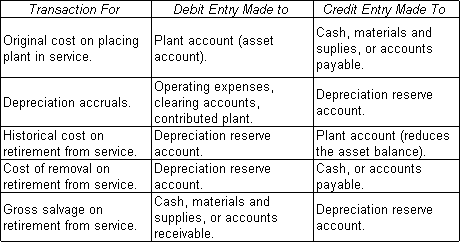
4. For complete details of the accounting transactions relating to depreciation reference should be made to the appropriate uniform system of accounts for the utility under study. As a reference in using this practice, the following tabulation presents in a broad way the essential transactions:
Definitions of Depreciation
5. The National Association of Railroad and Utilities Commissioners used the following definition: (NARUC Depreciation Committee Report of 1943 and 1944.)
"a. Depreciation is the expiration or consumption in whole or in part, of the service life, capacity, or utility of property resulting form the action of one or more of the forces operating to bring about the retirement of such property from service;
"b. The forces so operating include wear and tear, decay, action of the elements; inadequacy, obsolescence, and public requirements;
"c. Depreciation results in a cost of service."
6. The Federal Communications Commission employs the following definition: (Uniform System of Accounts for Telephone Companies, June 19, 1935, p. 4.)
"'Depreciation', as applied to depreciable telephone plant, means the loss in service value not restored by current maintenance, incurred in connection with the consumption or prospective retirement of telephone plant in the course of service from causes which are known to be in current operation, against which the company is not protected by insurance, and the effect of which can be forecast with a reasonable approach of accuracy. Among the causes to be given consideration are wear and tear, decay, action of the elements, inadequacy, obsolescence, changes in the art, changes in demand and requirements of public authorities. "
7. Depreciation has been defined by the Supreme Court of the United States as follows: (Lindheimer v. Illinois Telephone Company, 292 U. S. 151, 167 (1934).)
"Broadly speaking depreciation is the loss, not restored by current maintenance, which is due to all the factors causing the ultimate retirement of the property. These factors embrace wear and tear, decay, inadequacy and obsolescence. Annual depreciation is the loss which takes place in a year."
Sinking Fund Method
8. While this practice has been limited to the straight-line remaining life method, it may be applied in principle to other methods such as the sinking fund method. The sinking fund method defers heavy accruals until late years of service life. Particular care must be exercised in the utilization of the sinking fund method to determine proper accruals because of the interest feature. An equivalent remaining life which corrects for mortality dispersion must be determined. This equivalent remaining life will normally be shorter than the true remaining life in group accounts because of loss of interest on early retirements and because units of the group with longer lives have lower present worth weighting in providing for the interest factor. The interest feature also causes the sinking fund remaining life accrual to fluctuate more than the straight-line accrual where changes in life expectancy arise. Where the reserve has been over accrued, the interest component of the accrual may be more than sufficient to meet the required additions to the reserve. Under these conditions a red or debit annuity portion of the accrual may develop which, combined with the interest component, gives the correct total accrual to recover the original costs.
CHAPTER 2
REMAINING LIFE AND TOTAL LIFE METHODS
The Two Methods
1. In depreciation determinations the life used for computing the accruals may be an estimated total life or an estimated remaining life of property in service. Where the total life plant has been used and original estimates prove inaccurate, excessive or deficient accumulations in the depreciation reserve frequently occur. To overcome this, the use of the remaining life principle has been adopted by many utilities. This practice describes the latter method. However, as a matter of information, a comparison between the two methods is presented in this chapter.
The Total Life Equation for Depreciation
2. The basic formula for total life straight-line depreciation is:
d = (1 - c)/L
where
d = total life straight-line depreciation rate
c = average net salvage ratio (gross salvage less cost of removal) during total service life
L = total service life of unit or average service life of group of units
3. Thus a steel transmission main for natural gas is constructed at a cost of $100,000. A total life of 20 years with 10% net salvage is estimated. The depreciation rate is:
d = (1 - .10)/20 = .045 or 4.5% per annum
The annual accrual is $100,000 X 4.5% or $4,500.
4. Assuming that no additions to gross plant have been made and that there have been no interim retirements, the depreciation reserve accumulated for this line would at the end of 10 years amount to 45% and at the end of 20 years would amount to 90%, just sufficient to retire the line if net salvage equaled 10%.
Reappraisals of Depreciation Charges
5. Depreciation charges even in the simplest projects should be re-examined from time to time. It is obvious that, until final retirement, depreciation charges involve estimates of future life and salvage. What steps are taken on reappraisal of these estimates?
6. Continuing with the example of the natural gas transmission line, several conditions can be visualized upon reappraisal after, say, 10 years' time has elapsed. One condition may be to reaffirm the view of 10 years ago that the line still has a total life of 20 years and net salvage of 10%, in which ideal case no change in rate is necessary.
7. It is conceivable that the gas line will have a remaining life of only five years, giving a total life of 15 years. On the total life basis, the new rate
d = (1 - .10) / 15 or 6%
Accruals thus will total $45,000 for the first 10 years and $30,000 for the final five years or a total of $75,000. The reserve will be $15,000 deficient, assuming the line to be retired at the end of the fifteenth year and salvage of $10,000.
8. On the other hand, the reappraisal may indicate a relatively longer life and that the line with suitable repairs or replacements may last 30 years. The new total life rate then becomes
d = (1 - .10) / 30 or 3%
Accruals in this case include the $45,000 for this first 10 years and $60,000 for the remaining 20 years or a total of $105,000. With the salvage of $10,000, an over accrual of $15,000 would exist in the reserve at time of final retirement.
Total Life Theory Inadequate
9. Thus the reappraisals indicate that unless the original estimate of total life proves entirely accurate the total life concept fails to accomplish the solution of the basic problem of charging the cost of fixed capital (less estimated net salvage) to expense over its useful life, and deficits or excesses can arise by reason of changes in service life characteristics or changes in causes of retirement.
The Remaining Life Equation for Depreciation Rate
10. The remaining life straight-line depreciation method is designed to ratably recover the cost of plant, less net salvage and less depreciation reserve, over the remaining life of plant. The formula for this procedure is:
d' = [(1 - c') - u'] / E
where
d' = remaining life straight-line depreciation rate
e' = average net salvage ratio for remaining plant units
u' = ratio of depreciation reserve to original cost
E = future life expectancy of unit or average expectancy of group of units
11. In the reappraisal in the case of the shorter (15-year) life, the rate becomes
d' = (1 - .10 - .45) / 5 = .09 or 9%
thus accumulating $45,000 in the remaining five years, or a total of the desired $90,000.
12. For the longer (30-year) life, the rate becomes
d' = (1 - .10 - .45) / 20 = .0225 or 2.25%
and again the accumulation of $45,000 in the remaining 20 years, or a total of the desired $90,000.
13. These conditions are illustrated in the following chart:
(insert scanned chart)
CHAPTER 3
FACTORS INFLUENCING DEPRECIATION ACCRUALS
General
1. Several factors influencing depreciation accruals will be reviewed before considering the actual depreciation accrual. These factors are pertinent to a complete review of depreciation practices of a utility and should be considered by the staff engineer in preparing a report.
Accounting for Plant Additions and Retirements
2. The depreciation computations are normally based on the cost of property recorded on the company's books. Proper accounting records of plant are therefore important. The following points should be checked:
a. Are proper accounting entries, including charges to the depreciation reserve, made when plant is taken out of service?
b. When replacements of units of property are made, is the old unit retired and the new unit recorded as an addition to capital?
c. Have past service lives and salvage estimates been adjusted for changed conditions as new experience has been developed?
d. If old equipment has been continued in service beyond its normal retirement date as a temporary expedient to meet growing service demands, have adjustments to the depreciation rates been applied?
3. Application of the remaining life principle consistently applied over a period of years in connection with a depreciated rate base will normally tend to produce equitable results in rate proceedings even if these points have been incorrectly determined. Nevertheless, it is desirable to stress the maintenance of proper basic plant records.
4. Where feasible, it is desirable that the utility record the dollars in major accounts by year of placement, and relate retirements to the year of placement. This information is necessary where actuarial studies are contemplated in determining estimates of service lives. Such studies are desirable for large groups of property or where the total investment in an account is large. This information will also afford an age distribution of the dollars of plant by year of placement which data permits more accurate determination of remaining lives. These items are discussed in more detail in Chapter 5.
Retirement Pricing and Unit Prices
5. In large group accounts where it is impractical to determine actual costs of each item retired, average unit costs are often used. Determination of unit costs is facilitated if age distribution data are available. Inaccuracies in estimating unit costs or inaccuracies from other causes in pricing retirements, result in distortion of the gross plant and depreciation reserve accounts. While the remaining life method will tend to correct these inaccuracies, it is nevertheless important to obtain reasonable accuracy in the unit retirement costs applied to group accounts.
Unit and Group Bases for Accounting
6. The manner in which the depreciable plant is divided to form the bases on which the accruals are computed is an important factor in the depreciation computation. Where individual property units comprise the base the method is spoken of as unit accounting. Where groups of property, such as an entire account, comprise the base, the method is spoken of as group accounting. The accrual computation presented in Chapter 4 may be used with either base, provided appropriate unit or composite group values for salvage and remaining life are selected. The differences between the two bases may be summarized as follows:
a. Unit accounting (sometimes called item accounting) requires a specific record, usually a card, for each individual item of property. A service life and salvage estimate are applied and an individual accrual for the unit is determined. The accruals are accumulated each year on the unit record and reappraisals using the remaining life principle may be made. If the unit is retired ahead of its expectancy, the deficiency in accruals is charge to depreciation expense that year. If the unit outlives its expectancy, the accruals are stopped when the accumulations equal the full original cost installed less estimated net salvage, and no further accruals are made for that unit.
b. In group accounting all units having like mortality characteristics or all units of an account are considered together. Accruals for the group are based on composite or weighted average values of salvage and service life expectancy. The resulting values are applied to the surviving plant balances each year or each accounting period. A deficiency due to early retirement of a particular unit is made up through greater accruals on a unit which outlives the average. As discussed in Chapter 8, periodic reappraisals of the life expectancy and salvage estimates are required with group accounting. Because of greater simplicity in maintaining records, the group basis is more feasible for most classes of utility property where large numbers of units are involved. It is the more generally used base among electric, gas, telephone and water utilities.
Subaccounts of Plant, Classes of Property and Age Groups
7. To facilitate service life estimates in group accounting or to distinguish between certain recognized parts of a large account, subsidiary data showing subdivisions of an account are often maintained. These include the following:
a. Subaccounts are generally used to separate geographic portions, or where an account is large, to separate certain classes of property. For example, a telephone utility may separate Ac. 264, Vehicle and Other Work Equipment, into Ac. 264-1, Vehicles, and Ac. 264-2, Work Equipment. Where subaccounts have been established they are usually carried separately on the company's books and are thus treated as separate accounts in computing depreciation expenses and in recording reserves.
b. Classes of property are portions of an account having different physical or mortality characteristics. For example, a water utility may maintain data to show the portion under Ac. 343, Transmission and Distribution Mains, consisting of asbestos-cement mains, cast-iron mains and steel mains. To the separate classes of property, different service life and salvage estimates may be applied and a composite value for the account may then be derived as discussed in Chapter 5. Separation by classes of property also facilitates determination of average unit costs. The classes of property considered separately are often varied from year to year. Extensive use of classes of property within accounts tends to nullify the advantages of group accounting. The presence of distinct mortality characteristics and the dollar values of plant are criteria which should be considered in deciding whether to maintain separate data for particular classes of property. As a general guide, accounts of less than $25,000 of plant for Class B and C utilities and accounts of less than $100,000 of plant for Class A utilities, need rarely be subdivided by classes of property merely for group depreciation calculations. Above these amounts the presence of distinct mortality characteristics or other factors should govern, where separation into classes of property is contemplated.
c. Age groups (also called generations or vintages) represent the survivors of all units of an account or a class of property installed during the same year or span of years. Maintenance of age group or age distribution data permits more accurate determination of service lives and aids in applying unit retirement costs. For most types of mortality studies age group data are essential. Where large growth in an account has occurred and an initial subdivision is proposed, subdivision by age groups is usually preferred over subdivision by classes of property. Class A utilities may find both subdivisions desirable for major accounts.
Inventories and Appraisals
8. Where an inventory and appraisal of the property of a utility has been made, it may be desirable to adjust the books to record the appraisal and related depreciation reserve or to reach some agreed upon restatement in the light of existing facts as a preliminary step in adopting the remaining life method. In such cases appropriate authority of the Commission is needed, and any recommendation to adjust a reserve must be very carefully considered. As discussed in Chapter 4, the book reserve is ordinarily used, but if a restatement of the plant accounts has been approved, the corresponding restated reserve should be used. Once a reserve has been adopted for remaining life method, it should never again be adjusted except to correct accounting errors.
Historical Development of Depreciation Reserve
9. In preparing a report of depreciation practices of a utility, a historical review of past methods of determining credits to the reserve is often helpful. Where initial application of the remaining life method is being made, the considerations of Paragraphs 8 and 9 of Chapter 4 apply. It will be noted that ordinarily the book reserve should be retained and carried forward.
Maintenance Practices and Depreciation
10. In determining the service life of utility plant there is an inherent relationship between maintenance practices and depreciation. By increasing maintenance expenses the service life may often be prolonged, thereby permitting reduced annual depreciation expense. While no exact measure of this relationship is, of course, possible, it is well to inquire into the general level of maintenance when reviewing a utility's depreciation practices. Large maintenance programs will indicate longer service lives are more appropriate while the lack of maintenance program will tend to indicate that lives somewhat shorter than those for otherwise comparable properties would be appropriate. Maintenance practices also affect depreciation when replacement of smaller parts of a major plant unit are made. In a particular account as between two utilities, different service lives for otherwise comparable property will be indicated, if one charges all such replacements to maintenance while the other uses great refinement in retirement units and treats replacements of many smaller units as capital replacements. The latter condition tends to produce shorter service lives for the account, all other factors being equal.
CHAPTER 4
THE REMAINING LIFE DEPRECIATION ACCRUAL DETERMINATION
General
1. This chapter presents the basic steps in determining the straight-line remaining life accrual as of a given date, usually the first of the year, and discusses the source of each element in the accrual equation. Detailed information pertaining to methods of obtaining the element of remaining life expectancy is presented in Chapter 5. Procedures for advancing the determination through the year to cover additions and retirements and for applying the determination in succeeding years are presented in Chapter 8.
The Accrual Equation
2. The basic equation for the straight-line remaining life accrual is:
D' = (B - C' - U') / E
where
D' = the annual accrual in dollars
B = the beginning-of-year plant balance
C' = the estimated future net salvage in dollars
U' = the beginning-of-year book depreciation reserve
E = the estimated remaining life expectancy of the plant in years
as of the beginning of the year
It will be noted that the element B and U' are normally obtainable from the utility's books while the element C' and E require estimates of future conditions. These estimates should be reviewed periodically as discussed in Chapter 8.
The Standard Form for the Accrual Determination
3. The standard form for the accrual determination is illustrated in Tables 4-A to 4-E which show the complete determinations for typical utilities. This form is available with ruled lines (Form D-1) for work sheet purposes or in the plain style (Form D-2) for finished typing. The form is designated as an annual determination since the results represent an annual accrual or rate.
4. The numbered columns on the form show the elements B, C', and U' of the basic accrual equation in Columns 1, 2, and 3. Column 4 headed "Net Balance" shows the numerator of the equation, Column 5 shows the remaining life expectancy E. The accrual is then computed and shown in Column 6. The lettered columns on the form give supporting information sometimes used in developing the estimated values. Under group accounting a separate line is used for each account or sub account. Under unit accounting a separate line is used for each unit or group of similar units. Ordinarily the accuracy of estimates in the accrual determination is such that the entries may be rounded to the nearest dollar.
Plant in Service
5. The dollars of all depreciable plant in service at the beginning of the year as taken from the utilities' books are used in the accrual determination and entered under the heading "gross plant" in Column 1 of the standard form.
Future Net Salvage
6. Future net salvage as included in the accrual equation represents an estimate of the dollars which will be realized from the future retirement of all units now in service. Net salvage is gross salvage realized from resale, re-use or scrap disposal of the retired units less cost of removal. It is customary to arrive at the net salvage in dollars by applying an estimated percentage to gross plant. Column A of the standard form provides space for entering the estimated percent. The amount in dollars in Column 2 is then the product of the percent in Column A times the plant in Column 1.
7. In estimating the percent net salvage, past experience, when available from the accounting records, should be determined before arriving at a final estimate. However, future conditions often change materially from the past experience because of reduced salvage value of older units or changed conditions in the salvage market or in costs of removal. Also, the past retirement experience of most utility plant is based on but a small portion of today's existing plant. For estimating purposes it is often desirable to consider gross salvage and cost of removal separately. As a rule, gross salvage fluctuates with changes in material costs whereas cost of removal fluctuates with changes in labor expense. Where cost of removal is high, it may be economical, if practicable, to merely abandon plant, which consideration should be reflected in the estimates. It is the usual practice to develop one estimated percent net salvage value for all like units of property. If, however, there is a difference in characteristics or different market demand for units of different ages, the possibility of separate salvage estimates for different age groups should also be considered. When separate estimates are developed for different classes of property or different age groups, the composite estimate for the account should be determined by direct weighting. That is, by multiplying each percent estimate times its related dollars of plant, totaling these products and dividing by the total plant dollars. This gives the composite net salvage expressed as a ratio or a percent. Further detail on procedures used to assist in making salvage estimates is presented in Chapter 7.
Book Depreciation Reserve
8. The dollar balance in the depreciation reserve at the beginning of the year as taken from the company's records should, except in unusual cases, be entered in Column 3 of the standard form and be used in the accrual determination. This book reserve should be retained and carried forward each year by accounts on the remaining life basis. For companies having generally more than $100,000 of gross plant, where the reserve has not been maintained by accounts, the initial application of the remaining life method will require an allocation of the reserve by primary accounts. Companies with less than $100,000 of plant may, as an alternative, compute an over-all composite accrual as described in Paragraph 12 below.
9. An allocation of the reserve by accounts if required should be based on prorating the book reserve according to the reserve requirement or upon a historical reconstruction of the reserve for each account where records are available. If the reserve has previously been kept by groups of accounts or by departments, the allocation to accounts should be made within the group or department without disturbing these subtotals. It will be noted that a reserve requirement study is not required once the remaining life method is started and carried forward. Reserve requirement studies will not be made by the staff, except for the initial allocation to primary accounts, or except in special cases recommended by the Branch Engineer and approved by the Director or Assistant Director of the Utilities Division. Details of procedure when a requirement study is to be made should be reviewed with the Staff Advisory Section.
Remaining Life Expectancy
10. The remaining life in years to be entered in Column 5 of the standard form represents the composite remaining life expectancy for all units, age groups, and classes of property of the account at the beginning of the year. A determination of this value may be made by any one of several methods. The choice of method depends on a number of factors, particularly upon the data available from accounting and engineering records and upon the practical aspects of time and work economy. Details of the various methods and their applicability are discussed in the next chapter. Where the remaining life is determined directly, no entries need be made in Columns B, C or D on the standard form. Where the remaining life is determined from estimates of other service elements the latter should be entered in the appropriate columns.
Depreciation Accruals
11. Having completed entries in Columns 1, 2, 3, and 5 of the standard form, the annual accrual for conditions as of the first of the year may be computed as indicated on the form. It may be used directly as the total accrual for the year or may be adjusted for plant additions as discussed in Chapter 8.
Alternate Accrual Determination for Small Utilities
12. Utilities having generally less than $100,000 of total plant, who elect not to separate the reserve by accounts as discussed in Paragraph 8 above, will have but one total entry in Column 3. Under these conditions, it is appropriate to develop a composite value for remaining life for the entire plant. The total accrual is then obtainable by completing the determination across the totals line only on the standard form. The two alternate examples of Tables 4-D and 4-E illustrate the solution.
13. To develop a composite value of the remaining life from separate estimates by accounts, reciprocal weighting may be used as an approximation as follows:
a. For each account divide the plant in Column 1 by the remaining life in Column 5.
b. Total these quotients for all accounts and divide into the total of Column 1. This is the weighted composite remaining life.
14. Further simplification for utilities having generally less than $25,000 of plant may be made by omitting estimates for each account and developing by direct judgment a remaining life estimate for the entire plant.
(insert 5 pages here)
CHAPTER 5
METHODS OF ESTIMATING THE REMAINING LIFE EXPECTANCY
General
1. There is presented in this chapter: first, material on the general nature of remaining life estimates and plant mortality; second, the types of data available from which remaining life estimates may be developed; third, methods of weighting and a discussion of the factors governing the selection of a method; fourth, a brief presentation of the available methods of estimating remaining life; and, finally, a discussion of the governing factors and procedures in the selection of a method. Each of these items comprises a separate section of the chapter. Those familiar with depreciation practices, or those interested in an over-all picture, only, may wish to turn directly to the final section commencing at Paragraph 18.
A - REMAINING LIFE AND PLANT MORTALITY
Basic Nature of the Remaining Life Estimate
2. Determination of the remaining life basically involves the judgment estimate of the engineer as to the future effect of wear and tear, decay, action of the elements, inadequacy, obsolescence, and public requirements. In special cases other factors may be important, such as anticipated changeovers to new or improved major units of plant, and other specific plans of management. To arrive at a satisfactory estimate of future conditions, the past experience generally gives indications which may be used as a major element in the remaining life estimate. The weight to be given past experience depends upon the extent to which conditions affecting service life in the future are expected to be similar to or different from those in the past. However, substantial weight is generally given to results of past experience in the same or comparable properties.
Plant Mortality Experience
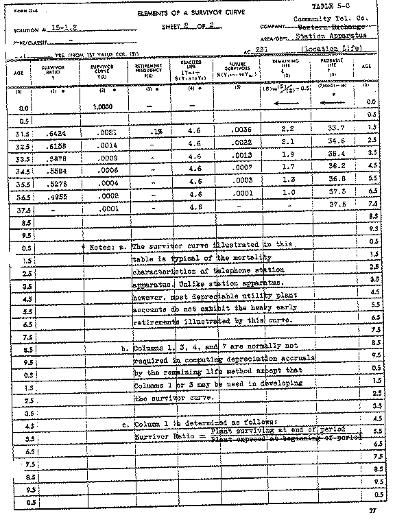
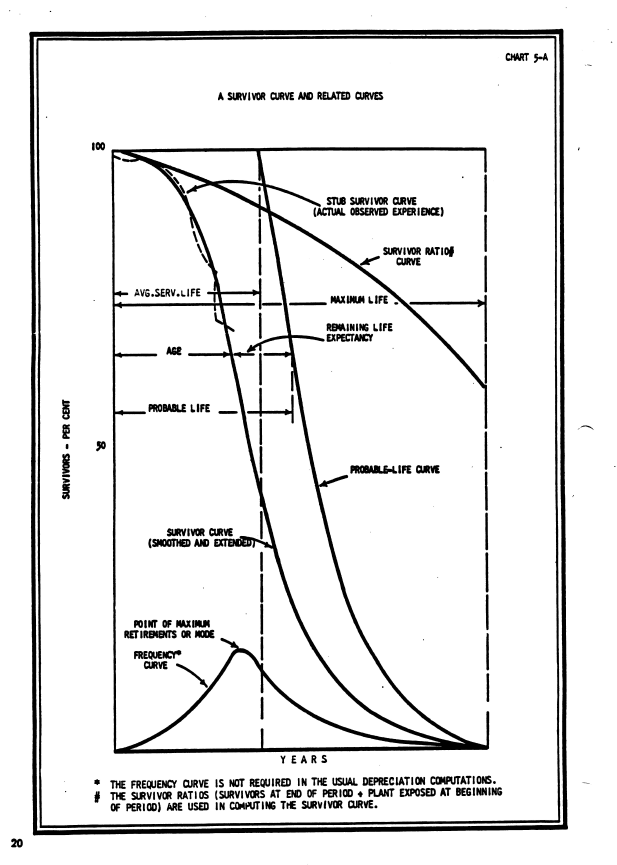
3. From the numerous studies of utility properties made by many individuals and organizations under widely varying circumstances, it is known that large groups of like plant generally follow a mortality pattern. This pattern is such that the portion of an original group surviving at a time may be statistically predicted as a function of age. A graph or curve illustrating this relationship is known as a survivor curve. Chart 5-A illustrates a survivor curve together with various related curves and service life elements. The more important service life elements include the following
a. Average service life is the average expected life of all units when new. It is also spoken of as the total service life of an original group as used in Column B of the standard calculation form D-2. It is equal to the area under the survivor curve and is illustrated by the vertical dotted line in Chart 5-A.
b. Probable life is the total expected service life of survivors at a given age. On the standard calculation form it may be entered in Column C. At any age beyond zero it is longer than the average service life by reason of retirements of shorter lived units which have already taken place.
c. Remaining life expectancy is the future expected service in years of a survivor at a given age. For single units or single age groups of property the age of the survivors plus the remaining life equals the probable life. Using this relationship the probable life curve is drawn so that for any age along the survivor curve the horizontal distance to the probable life curve represents the remaining life. For groups of different ages or different classes or property a weighted average expectancy is required.
d. Average age is the weighted average age of all units of plant in service at the beginning of the year. It may be entered in Column D on the standard calculation form. Use of this element to obtain the remaining life of group accounts involves an approximation which should only be used when other means are not available.
e. A stub survivor curve represents the observed experience for a particular account or class of property. A curve developed by statistical analysis or selected as a mean of observed experience is spoken of as a "smoothed" curve. Often observed experience does not extend to older lived units. Under these conditions the predicted experience for older lived units is spoken of as an "extended" curve. Generally a curve developed or selected for estimating purposes is a curve which has been both "smoothed and extended"
B - DATA AVAILABLE FROM UTILITY RECORDS
Sources of Data
1. Data available from utility records affording information on which to base estimates may be found among the following sources:
a. Accounting records in compliance with the "Uniform Systems of Accounts."
b. Parcel or card records of lands, buildings, structures, and other plant units.
c. Construction work orders and voucher records.
d. Engineering or operating maps, diagrams, and field records.
e. Data compiled to determine average unit costs.
f. Subsidiary depreciation records including mortality summaries, age and dollar distribution data, and retirement data.
2. Each of these sources should be checked with a view toward arriving at all available pertinent information. The more important types of information to be assembled as a basis for estimating lives are discussed in the next five paragraphs.
Mortality Summary Data
3. The mortality summary of an account or class of property provides the most reliable source for developing past results and statistically predicting future experience. Such a summary sets forth the dollars or units of plant placed each year and shows the related retirements by age at retirement. This information, when not maintained directly, may frequently be developed by study from those sources listed under Items b, c, d, and e in the preceding paragraph. In order to maintain this information it is necessary to record the dollars in each account by year of placement and relate retirements to year of placement. Where the group comprises many small units, this is sometimes accomplished by studies of representative samples. For accounts or single classes of property with over approximately $100,000 in plant, the accumulation of this data when at all feasible is recommended.
4. From the mortality summary, using actuarial methods, smoothed and extended survivor curves applicable to the plant in question may be developed. Available alternate methods of solution of the data include both the stub survivor curve directly, selecting a type curve by matching with the stub curve, smoothing the observed survivor ratios or retirement ratios, and smoothing the observed frequency curve. These various elements are illustrated in Chart 5-A. Complete details for using these methods are beyond the scope of this practice. Where data are available and the staff is to determine a solution, assistance of the Water Advisory Branch should be obtained. Where review of a utility's solution is made, the reasonableness of the band of years of past experience selected as representative of future conditions should be checked.
Distribution Data
5. Distribution data, when available, permits accurate development of remaining life from a selected survivor curve. These data show the dollars of plant surviving separated by age groups. Where mortality summaries are maintained, these data may be taken direct from the summary. In other cases, although mortality summary data are not available, age distribution data may be developed. This can be done by (?) from accounting records based on known placements or retirements of major units coupled with a first-in first-out treatment of unidentified additions and retirements. The first-in first-out treatment of additions and retirements is to be used with caution, particularly if applied to an entire account, for it distorts the mortality dispersion experience. An alternate and perhaps more accurate means of initially developing distribution data is to select an applicable survivor curve and apply the portion surviving for each age to known gross additions each year. The first four columns of standard form D3 provide for this calculation as illustrated in Table 5-A. When an age distribution study has been made, it is desirable if feasible, that all information thereafter be carried forward annually, particularly for accounts exceeding $100,000 in value.
6. Distribution data is sometimes used to determine age dollar and average age information. Determination of the remaining life of a group account by subtracting average age from an estimated average probable life is an approximation subject to possible wide error in results. Whenever a survivor curve believed reasonably representative of future condition may be selected, even if a type curve is selected on a judgment basis, the remaining life result, obtained by direct weighting as described below, is to be preferred over determining an average age and applying the group approximation.
(where are paragraphs 7 and 8?)
(insert two pages here)
Accounting Records of Gross Additions and Plant Balances
9. Where mortality summary data and age distribution data are not developed, considerable information on which to base estimates may be developed from the plant accounting records maintained in conformance with the uniform systems of accounts. Some caution must be exercised, however, to eliminate the distortion caused by transfers and adjustments to accounts, by changes in accounting classification, and by abnormally large retirements or replacements of units. Use of these data yields more reliable results in accounts with stable plant or plant with uniform growth where no noticeable trend toward longer or shorter service lives is evident. With these precautions in mind the following may be developed:
a. A representative survivor curve is obtainable by simulated plant balance methods.
b. Indications of average service life may be obtained by turnover methods.
c. From a selected applicable average service life indications of the remaining life may be calculated.
Details of procedure to accomplish items a and b are beyond the scope of this practice. Where a utility has used these methods, the staff engineer in his review should check the period of years used in relation to anticipated future conditions. He should also check to insure reasonable adjustment of the accounting data for transfers, changes in classification and other abnormal experience when applicable. Details of procedure to accomplish Item c are presented in Paragraph 16 below.
C - METHODS OF WEIGHTING
Types of Weighting
10. Before considering the methods for obtaining remaining life it is well to consider the means by which estimates for separate classes of property or separate age groups may be weighted to afford a composite value. Three types of weighting are used as follows:
a. Direct weighting or weighting by future dollar years. This calculation requires that the book dollars for each age group or class of property be multiplied by the remaining life applicable to those dollars. The composite remaining life is then obtained by dividing the total of the products by the total plant dollars. The products under this method of weighting are spoken of as future dollar years. The last three columns of standard form D3 may be used for this calculation as illustrated in Tables 5-A and 5-B.
b. Reciprocal weighting. This is accomplished by dividing the book dollars by the remaining life for each age group or class of property, totaling these quotients and dividing the total into the total book dollars.
c. Average service life weighting. In this method the book cost for each class of property is divided by the average service life and the result is multiplied by the remaining life. The composite remaining life for all classes then equals the sum of these products divided by the sum of these quotients.
Selecting a Method of Weighting
11. In selecting a method of weighting, several considerations apply. First, it is desired that the method of weighting used shall produce the same results as though the book reserve had been prorated to the various age groups or classes of property on the basis of the applicable reserve requirement. Secondly, it is desirable that the result obtained by weighting be in conformance with the provisions of certain of the uniform systems of accounts, that the accrual computed for an account as a whole shall be the same as if separate accruals had been computed for each class of property and the total obtained. Under these considerations, direct weighting produces proper results if the average service life of each age group or class of property weighted is approximately the same. Reciprocal weighting produces proper results if the reserve for the various classes of property or groups weighted is distributed in proportion to the plant dollars, a condition which is more likely in stable plant with slow growth. Average service life weighting produces proper results which is more likely in stable plant with slow growth. Average service life weighting produces proper results if the book reserve and the reserve requirement are closely the same. From these considerations it is concluded that direct or future dollar weighting is the proper method to use between age groups, whereas either reciprocal weighting or average service life weighting will usually yield the better approximation between classes of property. In very large accounts where individual classes of property exceed $100,000 of plant, occasionally a utility may prefer to prorate the book reserve within the account according to a reserve requirement between each class of property rather than to attempt any of the other weighting methods. Such a proration is used only infrequently, is made only at the time of a periodic review for weighting purposes within a very large account, and is normally not carried forward from the date of the calculation.
D - AVAILABLE METHODS OF ESTIMATING REMAINING LIFE
Survivor Curve Methods
12. If a survivor curve believed representative of future conditions can be developed or a type survivor curve is selected on a judgment basis, the determination of the remaining life is greatly facilitated. Standard form D4 provides for computing the elements of a survivor curve as illustrated in Table 5-C. Where mortality summary data are available, the curve should be developed from these data. Care should be exercised to select data from a band of years reasonably representative of the anticipated future conditions. In determining the shape of the extended portion of the curve, it is helpful to ascertain a reasonable maximum life or cutoff point for the curve. Other factors such as the operation of uniform chance retirement which produces a flat curve and the possibility of high early mortality which produces an early drop in the curve, or similar factors should be kept in mind. Usually it will be evident from the summary data that certain of these factors are operating in the plant and the calculated results will reflect these conditions.
13. When mortality summary data are not available the selection of a general type survivor curve is desirable. In selecting type curves the considerations enumerated in the preceding paragraph are applicable. Type curves may be obtained from actuarial analyses made of mortality data of comparable classes of property in comparable utilities or they may be obtained from general studies. One widely accepted study of this latter type is that conducted at the Iowa State College Engineering Experiment Station as described in their Bulletins Nos. 125 and 155. These curves are referred to in this practice as Iowa type curves. Tabulations of remaining lives by ages for each Iowa curve are given in the appendix. It will be noted that a particular type curve is identified by two elements. One is the average service life and the other is the type designator. The latter designates the general shape of the curve. When selecting the survivor curve on a judgment basis, the average service life must be estimated and an appropriate survivor curve shape selected. Turnover studies or related experience in other properties offer a guide to selecting an average service life. As a guide in selecting Iowa type curves, "L" types designate curves indicating high early mortality, "S" types designate curves with maximum retirements occurring about the mid-span of years, and "R" types designate curves with few early retirements and heavy retirements near the end portion of the curve. For each of these groups the higher subscripts indicate progressively greater concentration of retirements at one period.
14. Another method of developing a survivor curve is the simulated plant balance approach which involves a mathematical selection of that survivor curve which applied to the gross addition year by year will match the recorded year by year balances of the plant account. This method is applicable only where it is determined that past mortality experience has been consistent between generations and is reasonably indicative of the future. It is not applicable to plant accounts where substantial technical changes in the facilities have occurred. Two procedures have been advanced for developing the "simulated" balance solution. One procedure involves the successive trial of a number of curve patterns applied to the known additions to select the curve which most closely matches the actual plant balances. A complete discussion of this procedure using a set of precalculated tables based on the Iowa type curves is found in the paper entitled "Life Analysis of Utility Plant and Depreciation Accounting Purposes by the Simulated Plant Record Method" by A. E. Bauhan. The second procedure involves the use of the actual plant balances in the development of an equation for an approximate survivor curve of a predetermined generic type. A complete discussion of this procedure is set forth in a paper entitled "Mortality Curves for Physical Plant" by J. F. Brennan. Copies of these papers are in the Commission staff files (Staff Advisory Section).
Forecast Method
15. In certain accounts such as buildings, structures, telephone central office, dams, reservoirs, generating plants and other classes of property comprised of major units which it is expected will be retired as a single unit at one time, the development of an appropriate remaining life is more readily accomplished by direct estimate. This method is referred to as the Forecast Method or in some cases, the Life Span Method. The tabulation below shows a sample calculation using this method. First step in the procedure is to list each major unit of property included in the account together with its relating plant dollars surviving today (Columns 1 and 3). Next, a direct judgment estimate is made of the remaining service span or the terminal date when each unit will be retired (Columns 4 and 5). To the remaining span a small correction is applied for so-called "interim retirements" of smaller units comprising part of the major unit. Interim retirements and additions include such items as changes within a building or changes at an electrical generation station not altering the basic structures, etc. As an approximation the assumption is made that future annual interim retirements will occur at a consistent ratio to the present plant balance (Column 6). The correction for interim retirements is then developed by picturing the resulting survivor curve shape. The major unit of property with its forecasted terminal date is represented by a square-shaped survivor curve. The interim retirements cause the top of this square to slope downward to the terminal date when the entire unit is retired. The correction for interim retirements is then the area of the triangle lost at the top of the square by reason of the interim retirements. The base of this triangle is the remaining span. The depth (height of this triangle) is the interim retirement rate times the number of years during which they will continue, namely, the interim retirement rate times the remaining span. The correction for interim retirements (Column 7) is then the area of this triangle, or one-half times the interim retirement rate times the remaining span squared. In more accurate applications, this correction may be developed from an actuarial analysis of mortality data for the interim retirements. After applying the correction to obtain the effective remaining life (Column 8), the composite remaining life for the account is obtained by direct weighting with the dollars for each unit (Column 9). However, average service life weighting is more appropriate where only a few items occur in an account and a long time interval exists between the extreme probable retirement dates.
Approximation Method
16. Where survivor curves cannot be selected and the forecast method is not applicable, indications of remaining life may be obtained from the accounting records of gross additions and plant balances. Standard form D-5 provides for calculation by this method as illustrated in Table 5-D. The method is subject to the limitations discussed in Paragraph 9 above. However, indications may be obtained from a short span of years thereby avoiding some of the inconsistencies occasionally found in accounting data. Referring to Table 5-D, to apply the method, the starting plant balance, Item (4), plus the total gross additions (1) for a span of years is totaled to give plant exposed (6). The total of the plant balances (3) less one-half the beginning balance (5) and less one-half the ending balance (8) for the same span of years is likewise totaled (10) and a correction for past dollar years for transfers (11) is made to obtain Past Dollar Years (13). The quotient of these two totals [(13) divided by (6)] represents the realized life (14) of the plant during the span of years selected. The plant surviving at the end of the span (7) divided by the total of gross additions (6) indicates the portion of exposed plant surviving (9). The remaining life (16) has been obtained by selecting an appropriate average service life (12), subtracting from this the realized life (14) and dividing this difference (15) by the portion surviving (9).
When using this method where heavy additions to plant have been made in recent years, it is unnecessary to extend the span of years beyond the beginning of the heavy additions to derive reasonable indications of the remaining life. Where consistent accounting data is not available prior to a given year, this will determine the starting balance. If the starting balance under these circumstances is sizable, an estimated correction to the past dollar years for the prior life of this plant is required.
Direct Judgment Method
17. Where lack of appropriate data and other considerations make the application of any of the preceding methods unavailable, direct engineering judgment estimates of service life expectancies may be appropriate. It should be helpful to the engineer to study possible ranges of life estimates, setting down reasonable minimum and maximum expectancies before coming to final conclusions. Likewise, where the judgment method is being used, it may be desirable to consider the relationship of age plus remaining life which equals probable life. As previously noted at any age the probable life of survivors equals the age plus remaining life expectancy. This relationship is strictly true only for groups with all units of one age whose probable life is correctly estimated. However, the relationship is of value in determining a judgment estimate of remaining life. It should be noted that the average life of all units originally placed in the group, is less than the probable life of surviving units because of the prior retirement of short-lived units.
E - CHOOSING A METHOD OF ESTIMATING REMAINING LIFE
Steps in Choosing a Method
18. As can be seen from the foregoing, the methods available for estimating remaining life range in detail and accuracy from full actuarial analysis with age group weighting, through various approximation methods, to the simple direct judgment selection of a value for "E". In choosing a particular method best suited to the property in question the engineer should first have in mind the general nature of plant mortality characteristics and pertinent experience in similar properties; second, he should determine the type data available from the utilities' records; third, he should evaluate available methods in relation to the size of plant and the practical aspects of accuracy and work economy; and, finally, consistent with all the foregoing, he should select a method designed to yield the greatest accuracy practicable. Oftentimes it may be desirable to use different methods for different accounts and sometimes even for different classes of property within the same account. These steps are discussed in detail in the remaining paragraphs of this chapter.
Step One: "Have in mind the general nature of plant mortality characteristics and pertinent experiences in similar properties."
19. Paragraphs 2 and 3 of this chapter provide a basis for this information. Also the staff engineer should review recent depreciation studies of comparable utilities, and make a field inspection of the properties. For the larger utilities, experience in comparable accounts of the same utility should be noted. Other background information on mortality characteristics is covered in Chart 5-A and in Chapter 6.
Step Two: "Determine the type of data available form the utilities' records."
20. Paragraph 4 enumerates some sources of data. Paragraphs 5 through 9 discuss types of data which may be assembled to aid in determining estimates. The various factors of Chapter 3 as applied to the utility in question are also pertinent. Particular attention should be given to the methods used in determining unit retirement costs or retirement charges. Often appropriate mortality summary or age distribution data may be assembled from the unit cost data. One further consideration should be undertaken in this step; namely, the base for individual estimates should be fixed. Thus the classes of property within each account should be considered and those to be treated separately in the estimates should be selected. The presence of district mortality characteristics and the availability of data to permit separate estimates are criteria to be considered in this selection.
Step Three: "Evaluate available methods in relation to the practical aspects of accuracy and work economy.
21. The available methods are described in Paragraphs 13 through 17 above. Certain methods, as indicated, require detailed technical knowledge for which qualified personnel may not be available to smaller utilities. Different degrees of approximation are involved in each method. Generally, the more approximate methods are easier to apply but are subject to greater possibility of error. Considering the methods solely form the standpoint of accuracy, the preferable methods may be enumerated in the following order:
a. Develop a survivor curve by actuarila analysis and apply direct weighting of age groups.
b. Develop remaining life by forecast methods.
c. Select a type of survivor curve from actuarial analysis of comparable property and apply dir4ect weighting.
d. Select a survivor curve by simulated plant balance methods and apply direct weighting.
e. Select a type curve on a judgment basis using turnover indications of average service life if available and apply direct weighting.
f. Use the method of approximation from plant account records
g. Determine remaining life by judgment means.
For accounts exceeding $100,000 in plant, development of the remaining life using type curves and direct weighting of age groups or more accurate means is urged. The last two alternatives, while applicable to any size account, are more appropriate for accounts of less than $25,000.
Step Four: "Select a method designed to yield the greatest accuracy practicable."
22. The final selection of a method will be somewhat apparent from the foregoing steps. Limitations on available data will result in deletion of some methods; smaller utilities will lack qualified personnel to perform some of the more accurate methods, etc. As a general guide, it is desirable to apply a survivor curve wherever possible. From a survivor curve weighting by age groups may be applied as illustrated in Tables 5-A and 5-B. The standard form for this calculation is designated Form D-3. Space is provided on the form for deriving age distribution data from gross additions and a selected survivor curve. Where the survivor curve is determined by actuarial analysis, or where age distribution data are otherwise available, Columns 2 and 3 of the form need not be used. Where the Iowa type curves are selected the appropriate remaining life to be entered in Column 5 may be taken from the tabulations given in the Appendix. To aid in testing the reasonableness of final results, some typical average service lives are given in Chapter 6. These typical results may be helpful, but they are to be used with caution.
23. The final selected value of the remaining life as previously discussed should be entered in Column 5 of the standard determination form D-1 or D-2. Where estimates of average service life, probable life, or average age were used to develop the remaining life estimate, these values should be shown in Columns B, C, and D of the standard determination form.
Choosing a Method for Smaller Utilities
24. The preceding discussion of the steps in choosing a method to be used for estimating the remaining life expectancy is applicable to utilities of all sized. However, smaller utilities having limited technical personnel available or having a minimum of records relating to plant additions and retirements, will find but one or two methods applicable. As a general rule, the utilities having less than $100,000 of plant must rely largely on the Judgment Method described in Paragraph 17. These utilities may also occasionally use the Forecast Method described in Paragraph 15.
CHAPTER 6
TYPE CURVES AND TYPICAL EXAMPLES OF
SERVICE LIFE ESTIMATES
Applicability of This Material
1. The material presented in this chapter is offered as an aid in formulating engineering estimates of service life expectancies. Application of these data to a particular group of properties must be based on knowledge of local conditions, company policy with regard to retirements and other factors influencing service life.
Ranges of Typical Average Service Lives
2. The following tabulations give ranges which have been selected a typical for values of straight-line average service lives used by utilities in California. Also shown is a suggested method for an average utility to use in estimating remaining lives of the indicated account.
Iowa Type Survivor Curves
3. There are presented in the tables in the Appendix the portions surviving and remaining lives by ages for various average service lives for the 18 type curves developed at the Iowa State College Experiment Station. Remaining life expectancies have been computed form the data given in Bulletin 125, 155 and 156 issued by the Iowa college. These curves are referred to as "Iowa" type curves or as "Winfrey" type curves. The former designation is adopted in this practice. The latter designation refers to Professor Robley Winfrey, author of these Iowa bulletins.
4. A tabulation indicating curve types found applicable to certain classes of plant is also shown in the appendix. The indicated applicability of these curves is, of course, only general in nature and is largely based on the experience of the Iowa studies. In particular instances, the engineer may determine other type curves to be more specifically applicable than these general studies.
5. The portions surviving shown in the Iowa tables may be used to develop age distribution data as illustrated in table 5-A, and the remaining lives shown may be used to develop a composite remaining life from age distribution data as illustrated in Tables 5-A and 5-B.
6. A more compete set of Iowa type survivor and average remaining life tables has been compiled by Edison Electric Institute and American Gas Association. The tables give survivors of an original addition of 1,000 and corresponding average remaining lives to the nearest tenth of a year at half-year ages from 0.5 to 74.5, inclusive, for average lives from 5 to 100 years, inclusive. The tables were computed for the familiar mortality dispersion curves listed in the Iowa Bulletins, for dispersion intermediate to those in the bulletins and for two other type curves, SC and SQ. The curve designated SC is the Patterson C type curve, having a uniform distribution of retirement form age zero to twice average life. The designation SQ is for the square type survivor curve which ahs no mortality dispersion, i.e., all retirements occur at average life(at terminal life).
CHAPTER 7
DETERMINATION OF GROSS SALVAGE
AND COST OF REMOVAL
1. The detailed procedures presented below are applicable to larger utilities or larger accounts where they may be used as an aid in arriving at estimates of proper future net salvage. This material supplements Paragraphs 6 and 7 of Chapter 4 which present the basic consideration. Net salvage is defined as gross salvage realized from resale, re-use or scrap disposal of the retired units less cost of removal.
Determining Recorded Salvage Experience
2. Where records are available recorded salvage experience for each account may be determined by analyzing the credits and debits to the reserve. To do this, total the retirements for each year and determine the corresponding totals of gross salvage and cost of removal. Dividing each of the latter by the retirements gives the percent gross salvage and percent cost of removal realized for each year. This calculation for a series of years is illustrated in the upper portion of the examples shown in Tables 7-A and 7-B using standard form D-6. In using this information for determining estimates it is often helpful to plot a graph of successive values each account, it may be desirable to make a determination for all accounts as a whole to test the over-all reasonableness of the various estimates.
Future Gross Salvage
3. In most classes of property the percent gross salvage realized on retirement varies with the age of the unit. Generally, the older units yield lower values. Past experience is usually based on but a few retirements, probably of shorter-lived units; therefore, future gross salvage will usually be less than the recorded experience. For very accurate determinations predicted salvage values by ages should be weighted with predicted retirements by ages. As an approximation, however, reasonable results may be obtained by assuming a straight-line diminution from realized gross salvage of early retirements to the predicted ultimate gross salvage of oldest-lived units. The sample calculation shown in part 2 of Table 7-A illustrates an application of this assumption. The past experience for a recent span of years is noted. Anticipated ultimate gross salvage of the oldest surviving units is then estimated and an average of these two values is selected as the anticipated future gross salvage applicable to today's plant. In predicting ultimate gross salvage of older-lived units for certain classes of property such as cable, wire, buildings, motor vehicles and similar items, market conditions in the future may influence the results more than any other factor. The engineer should use reasonable market predictions for the immediate future as though applicable throughout the property life. Corrections for long-term changes in the market may be made, if necessary, at the time of periodic reviews under the remaining life plan.
(skipped two pages)
Future Cost of Removal
4. As pointed out in Chapter 4, cost of removal is essentially a labor cost. Predicted future cost of removal should be based on a reasonable projection of recent experience reflecting anticipated changes in labor cost for the immediate future. Possible abandonments of plant, or changes in cost of removal when resale of a plant item is not planned, are future factors to consider.
Accounts With High Turnover and Re-use of Plant
5. In certain accounts, notable the station apparatus account of telephone utilities, the placement and retirement of property units may be recorded on a location basis while the actual unit is retained and used successively at several locations during its "fixed capital" or physical life. Under these conditions the net salvage is a composite of the value for retirements where re-use occurs and the value at final retirement. The composite estimate of future net salvage may be arrived at by weighting separate service life and salvage estimates as illustrated in the following example:
a. Values selected by estimate:
Average Service life (fixed capital) ...................................... 18.0 years
Average Service Life (location) .......................................... 4.6 years
Average Net Salvage re-use Retirement .............................. 94%
Average Net Salvage Final Retirement ................................. 8%
b. Derived Data:
Average Recorded Net Salvage for past year or recent years ... 84.3%
Portion which today's surviving plant represents of the original
plant from which it was placed (location basis) ................ 52.7%
(This may be derived from the selected survivor curve applied to age distribution
data or to recorded gross additions.)
c. Solution:
Average number retirements during capital life = 18/4.6 = 3.9
Average number re-use retirements = 3.9 - 1.0 = 2.9
Average net salvage during total life of original group =
[(2.9)(94) + (1.0)(8)] / 3.9 = 71.9%
Percent of Orig. Net Direct Group Salvage Weight
(1) (2) (3) = (1)X(2)
Whence:
Past Retirements 47.3 84.3 3987
Present Surviving Plant 52.7 C' C' X 52.7
Total Plant ........................100.0 71.9 7190
CHAPTER 8
CARRYING FORWARD THE ACCRUAL DETERMINATION
Problems in Carrying Forward the Accrual
1. The depreciation accrual determined from standard form D-1 or D-2 is based on plant balance, book reserve and remaining life as of the beginning of the year. For each account where a complete study has been made in developing this determination three problems arise in applying it to the utilities' books and carrying it forward. First, the accrual to record for the study year is needed. Next, it is necessary to consider the means of determining accruals in the intervening years before another complete study of the account is made. Finally, the length of period between complete studies should be considered, it being inherent in the remaining life method that periodic reviews of estimates and reappraisals to correct for changing conditions will be made. These three problems are discussed under separate subheadings below. However, before turning to these, there is first presented material on accounting procedures for crediting the accruals and determination of the depreciation rates which are applicable to the problems.
Accounting Procedures for Crediting the Accruals
2. Several methods for recording the accrual on the books of a utility at the time of a study are used. These may be summarized as follows:
a. Use the beginning-of-year accrual as determined on the standard form as the accrual for the year. This is the simplest and most straightforward means of recording the accrual. It may be done as a single entry for the year or in 12 equal entries by months.
b. Compute the recorded accrual using the beginning-of-year determination plus a correction for estimated net additions to plant to be made during the year. It is assumed that the one annual depreciation accrual figure will be determined and applied for the year either as one figure or in 12 equal portions monthly. The correction may be determined by applying a composite rate applicable to the entire plant, or if the estimated net additions have been developed separately by accounts, it may be determined by applying rates for each account to the estimates of additions. Normally class A utilities should make the estimate by accounts or functional groups of accounts. The amount to which the rate is applied should represent average net additions. It will be noted that as an approximation net additions may be assumed to take place at the mid-point of the year; hence, one-half the total estimated net additions may be used as the average net additions. An illustration of the use of the composite rate applied to estimated net additions is shown in Table 4-A. Corrections for actual average net additions should be applied at the end of the year when final values are obtainable.
c. Compute the accrual on plant balances other than the beginning of the year balance. This requires first determining a depreciation rate and then applying the rate to the appropriate plant balance. Variations of this procedure include: determining an accrual by applying rates to the average plant balance for the year, determining a monthly accrual for each six months on the January 1st and July 1st balances, determining accruals monthly by applying rates either to the average monthly balance or to the beginning of the month balance each month. In using these procedures, often estimates are made for the original entries and corrections are applied when final plant balances are known. Use of this method applying the rate to either monthly or average monthly balances is required of Class A and Class B telephone utilities.
d. Adopt the determinations as of the beginning of a study year as a base, and during the interim until a complete new study is made, maintain separate records showing this plant base less retirements on the one hand and additions since the study date on the other hand. To the one base the remaining life rates are applied and to the other a total life rate for a selected average service life is applied. This method requires a double recorded for each account thereby tending to defeat the advantages of group accounting. Furthermore, while this method is theoretically more accurate, its practical advantage is questioned unless wide difference between the reserves has developed. If the reserves are reasonably close as between the book figure and the calculated reserve requirement, then the total life rate and the remaining life rate are close in value. The corrective factor inherent in the remaining life method will correct for the small differences as periodic reviews are made. The staff will not use this method in its estimates and reports except under unusual circumstances which should first be reviewed with the Staff Advisory Section.
3. During intervals between complete depreciation studies, the methods used to determine accruals include the above methods carried forward plus some additional methods involving partial redeterminations from the basic estimates. The various alternatives may be summarized as follows:
a. Use the depreciation rates developed at the time of the study applying them to the new first of the year plant balances as in method a. above.
b. Use the depreciation rates developed at the time of the study applying these to the new first of the year plant balances plus estimated average net additions as in method b. above.
c. Use the depreciation rates developed at the time of the study applying these to plant balances as in method c. above
d. Continue the separate records of plant less retirements from the study date and additions since then, applying remaining life rates and total life rates to the two balances, respectively, as in method d. above. If carried forward more than a year or two, retirements from the additions must be considered. This method is not recommended for staff use.
e. Using survivor curves selected in the study, derive new remaining life estimates by direct weighting from new age distribution data and recompute the accrual using standard forms D-1 or D-2 for new beginning-of-year plant and reserves.
f. Using the service life estimates developed in the study, derive a new remaining life estimate by judgment method from new average ages of plant and recompute the accrual using standard forms D-1 or D-2 for new beginning-of-the-year plant and reserves.
Determining Depreciation Rates
4. The standard forms D-1 or D-2 for the accrual calculation provide space in Column E for computing the remaining life depreciation rate for each account. This rate is obtained by dividing the accrual in Column 6 by the plant in Column 1. It is usually expressed in percent, that is, as a percent of gross plant. The composite deprecation rate for the entire depreciable property is obtained by dividing the total of Column 6 by the total of Column 1.
Selecting a Method of Determining the Study Year Accrual
5. Ordinarily the staff engineer in reviewing depreciation practices of a utility will apply the accounting procedure currently used by the utility. However, where a procedure is being established or a change is indicated other considerations may apply. Briefly, method a in paragraph 3 above, is the simplest and is used by some large as well as some small utilities, methods b and c yield results based on average plant which conforms to the procedure used in determining rate base, while method d as noted above is not recommended. As between methods b and c, the latter is more applicable to larger utilities where monthly balances are available and greater accuracy may be desired. For smaller utilities, method b is recommended for staff use.
Selecting a Method for Determining the Accrual in Years Between Studies
6. When determining the accrual in the intervening years between complete studies of an account, methods a, b, and c of Paragraph 3 above, which use the depreciation rate developed at the time of the last study applied to new plant balances, yield reasonable results with a minimum of calculation. When selecting as between these three methods, the considerations discussed in the preceding paragraph apply. Where large changes in plant are taking place or where it is desired to extend the period before another complete study is made, methods e and f of Paragraph 3 involving partial re-estimates or recalculation are more appropriate. This is particularly true for larger utilities or for individual account exceeding $100,000 of plant.
Period Between Complete Studies
7. Depreciation charges even in the simplest project should be re-examined from time to time. It is obvious that, until final retirement, those charges involve estimates of future life and salvage. This is particularly true under group accounting where average and weighted values are used. The remaining life method requires reappraisals and reviews of the estimates used from time to time. Complete study of the basic data and new determinations of estimates should be made for each account at intervals depending upon the occurrence of changes in conditions which suggest change of characteristics of the account. Thus, wherever large additions or large retirements have been made, new studies in the subsequent year are indicated.
Where uniform or nominal growth continues through a span of years, periodic study of each account, according to the following scale is suggested:
Recommended Maximum Interval Between Studies | |||
Where Accrual in Intervening Years is Determined Each Year by: |
Accounts of over $100,000 of Plant |
Accounts of $25,000 to $100,000 of Plant |
Accounts of Less than $25,000 of Plant |
Applying depreciation rates to new plant balances (Methods a., b., c., Paragraph 3) |
2 years |
3 years |
4 years |
Applying new age distribution data from derived survivor curves to give new remaining lives and applying this to new plant and reserve balances (Method e.) |
4 years |
5 years |
5 years |
Applying new judgment estimates of remaining lives to new plant and reserve balances (Method f.) |
3 years |
4 years |
6 years |
Annual Reviews and Schedules of Studies
8. Large utilities are, in general, required to review depreciation accruals annually and file with the Commission annual reports showing changes in estimates or rates which management feels should be made together with the resulting accruals. In connection with these reviews it is suggested that periodic studies of a number of accounts be made each year, according to a predetermined schedule, so that over a span of a few years detailed studies of the entire plant are made. Suggested material to include in the review reports is a follows:
a. Preliminary report to be submitted by December 1st.
(1) A list of the accounts on which the company has made studies of the basic estimates of service life expectancies and salvage during the past year and the results of these studies. These results should show changes where applicable by accounts, and likewise should show those accounts for which it was determined after study that no change in basic estimates is required.
(2) Note any major additions or retirements which it is contemplated will be made during the ensuing year and which will result in sizable changes of the depreciation accruals.
(3) An estimate of the dollar effects by accounts, of the changes indicated in items (1) and (2) above.
(4) A statement that no substantial change is anticipated other than those indicated in items (1), (2) and (3) above.
(5) A copy of the company's current program for studying accounts (if previous reports of the program have been made the changes only need be indicated).
b. Final report to be submitted by April 15th. (Companies closing their books other than the first of the year may use a different date.)
(1) The plant balances of all depreciable property by accounts and by study group subaccounts as of the first of the year.
(2) The depreciation reserve balances as of the first of the year.
(3) The applicable estimates of future net salvage and remaining life as of the first of the year or depreciation rates which will be applied to compute accruals during the current year.
(4) The dollar accruals based on beginning of year plant or estimated average plant.
(5) Items (1) to (4) above may be presented on the standard accrual determination form D-1 or D-2.
(6) Where changes in the estimates presented in the preliminary report have been made these should be indicated.
9. Smaller utilities not filing annual review reports will more often combine their reviews with periodic studies of all accounts at one time. Such reviews should be made every three or four years, and in any event not longer than five years apart, depending on size and circumstances as indicated in paragraph 7 above. The results of these reviews shall be filed with the Commission.
CHAPTER 9
GENERAL CONSIDERATIONS AND STAFF PROCEDURES
Check List for the Staff Engineer
1. Chapters 3, 4, 5, and 8 of this practice have been arranged in the general order of approach of a staff engineer preparing the depreciation portion of a results of operation report for ratemaking purposes. Some additional pertinent considerations are included in this chapter to assist the engineer. A brief checklist of suggested staff procedure is as follows:
a. Examine the utility's books with reference to the plant accounts and the depreciation reserve. This step is discussed below.
b. Review the company's past and current practices affecting depreciation. This step is the subject of Chapter 3. Additional considerations are enumerated in Paragraphs 12 through 17 of Chapter 5 and also in Paragraphs 2 and 3 of Chapter 8.
c. Review the availability of records other than the accounting records which will assist in making estimates. This step is discussed in Paragraphs 4 through 9 of Chapter 5.
d. Set up the standard accrual form and enter the known book values. This step is the subject of Chapter 4.
e. Make estimates of salvage for the various accounts and classes of property. This step is discussed in Paragraphs 6 and 7 of Chapter 4.
f. Make estimates of the remaining life of each account. This step is the subject of Chapter 5.
g. Make a field inspection of the properties with a view toward testing the reasonableness of estimates as evidenced by physical conditions which may be observed.
h. Complete the accrual determinations as discussed in Paragraphs 11 to 14 of Chapter 4.
i. Carry the accrual determination forward for the year(s) covered by the report. This step is the subject of Chapter 8.
j. Prepare a report of depreciation reserve and expenses for inclusion as a chapter in the results of operation report. This step is discussed below.
Examination of a Utility's Books
2. In undertaking a depreciation study, the books of the utility with respect to the plant accounts and the depreciation reserve should be inspected and checked to assure that reasonable procedures have been used in arriving at the current values. The historical origin of the initial entries either on formation of the company, on outside appraisals, or on prior actions by the Commission should be checked and the accumulations since that date reviewed. If doubt as to the correctness of the original entries or if evidence of arbitrary write-ups or write-downs appears, the matter should be reviewed with the possibility of requesting the Finance and Accounts Division to undertake an audit. In connection with the depreciation reserve account, check for possible transfers to or from surplus. Where it appears that the accounting requires corrections, the accrual determinations should be deferred until these corrections have been determined. Approval of the Director or Assistant Director of the Utilities Division should be obtained if an appraisal and reserve requirement study for purposes of restating the books is contemplated. In recommending such a procedure specific reasons for doing so should be stated. All efforts to utilize recorded book figures (with adjustment, if necessary) without appraisals should be explored.
Special Considerations for Smaller Utilities
3. As previously noted in Paragraph 12 of Chapter 4, utilities having generally less than $100,000 total plant may simplify the accrual determination by using composite values rather than attempting separate results by accounts. For these utilities it is essential that two minimum conditions be met. First, the accrual should be determined as described herein, and credited annually to the reserve. This may be based on judgment estimates for very small utilities applied as a single percent to gross plant. Second, the retirements of plant should be recorded and deducted from both the capital and the reserve accounts. The staff engineer in viewing the depreciation practices with utility representatives should stress these two essentials in preference to presenting too much detail with regard to the depreciation determinations itself. Good engineering judgment in selecting over-all estimates to arrive at a composite rate may be the only practicable means of determining consistent depreciation charges for very small utilities.
Depreciation Charged Through Clearing Accounts
4. In larger utilities it is common practice to charge depreciation on such items as vehicles and work equipment to a clearing account from which the portion assignable to construction and the portion assignable to maintenance is later determined. Where clearing accounts are used, the engineer must set out separately the depreciation accruals which are charged to clearing. These accruals are not part of the charges to the depreciation expense account.
Preparation of a Staff Report
5. In preparing the chapter on depreciation reserve and depreciation expenses for a standard results of operation report, certain pertinent items from the engineer's study should be included. The nature of the original entries should be recited and a tabulation of the historical growth of the depreciation reserve should be shown. A weighted average book depreciation reserve for the years under consideration should also be shown. This may be determined as the mean of the beginning- and end-of-year balances, or the mean of average monthly balances where these are available. The weighted average depreciation reserve is carried forward to the rate base chapter for the reserve deduction. The depreciation accruals as recorded for a recent year and determined for the current year should be shown. Where the company has not previously used the remaining life method, the following paragraph should be included:
"Consistent with standard practice, the staff has adopted the remaining life basis for computing depreciation expenses. The remaining life method meets the basic objective of depreciation of recovering the original cost of fixed capital (less estimated net salvage) over the useful life of the plant by means of an equitable plan of charges to operating expense accounts. Periodic reviews inherent in the method give assurance of continuous reasonable depreciation accruals. "
A complete determination as prepared on standard forms D-1 or D-2 should also be included. Additional material which may be presented in larger company reports includes: A tabulation of company and staff estimates, a tabulation of the depreciation reserve by accounts as of a recent date, and a tabulation showing methods of allocations between divisions or departments. Further information in preparation of a report is contained in Standard Practices U-2 and U-3.
Analysis of Reasonableness of Results
6. In the final analysis, a determination of depreciation accruals is based on engineering judgment of anticipated future conditions. It is therefore well to apply some test of reasonableness to the final results. Normally the composite accrual rates for a company should fall somewhere in the range from 2% to 4%. Where a composite rate exceeding 4% develops, it may be well to check the estimates or to analyze company policies with regard to placement of new plant and retirement of old units. As a further test of the reasonableness, it is well to compare the results determined for rate-fixing purposes with those reported for income tax purposes. In particular, the depreciation reserve carried on the books as compared with the depreciation reserve carried for income tax purposes should be noted.
Depreciation for Income Tax Purposes
7. In computing the depreciation allowance for income tax purposes it is often feasible, particularly for small companies, to apply the same determination for both tax and rate fixing purposes. However, differences in such factors as use of beginning of year versus weighted average plant, charges for interest during construction, past credits and debits to reserves, and other factors may cause differences in the two determinations. For information regarding depreciation requirements for income tax purposes "Bulletin F" of the U.S. Treasury Department, Internal Revenue Service should be consulted.
Extraordinary Obsolescence
8. Occasionally instances of extraordinary obsolescence such as the unexpected early retirement of a major unit of property may require some form of an adjustment. When instances of this type arise, application of the remaining life method will often provide a reasonable accrual. If, however, in the opinion of the staff engineer, special consideration is required he should refer his recommendation in the matter to the Director or Assistant Director of the Utilities Division.
Standard Forms
9. To assist the staff engineers, standard forms have been prepared for recording data and calculating depreciation results. These forms as illustrated in this practice are as follows:
CHAPTER 10
COMPANIES USING THE REMAINING LIFE METHOD
General
1. Most of the large utilities in California determine depreciation accruals using the remaining life method. It is being employed as standard practice in small company rate proceedings, at which time provision is made for continuing the accrual on this basis. Thus over a period of time it is anticipated that most small utilities will determine accruals on the straight-line remaining life basis.
Larger Utilities
2. All large electric, gas, telephone and water utilities in California, with the exception of one, now utilize the remaining lfie basis for book depreciation accruals, as follows:
California Electric Power Company
California Interstate Telephone Company
California-Oregon Power Company, The
California-Pacific Utilities Company
California Water and Telephone Company
California Water Service Company
Citizens Utilities Company of California
Clear Lake Water Company
Dominguez Water Corporation
General Telephone Company of California
Kern Mutual Telephone Company
Pacific Gas & Electric company
Pacific Lighting Gas Supply Company
Pacific Water Company
San Diego Gas & Electric Company
San Jose Water Works
San Gabriel Valley Water Company
Sierra Pacific Power Company
Southern California Edison Company
Southern California Gas Company
Southern California Water Company
Southern Counties Gas Company of California
Suburban Water Systems
Sunland-Tujunga Telephone Company
Western California Telephone Company
3. Agreements have generally been reached with the larger utilities setting forth details of introducing the remaining life method. Where decisions have required the remaining life method, agreements have usually been reached as a basis for such decision. It is not possible to include a typical agreement since conditions differed to some extent in each case.
4. In general, the above companies submit annual statements of their depreciation accruals. Twenty-two of these companies use the straight-line method. Three use the sinking fund method with various interest rates.
Smaller Utilities
5. In general, agreements as such have not been entered with the smaller companies. The staff engineer as standard practice in rate proceedings in the "Results of Operation Report" generally determines the recommended depreciation accrual on a remaining life basis for rate-fixing purposes. If such allowance is approved by the Commission and allowed in the new rate level, the Commission normally includes a provision in the order as indicated below. At the present time over 300 smaller utilities are using the straight-line remaining life method.
Typical Wording of Ordering Paragraphs
6. Where the remaining life depreciation method has been ordered by the Commission, typical ordering paragraphs have been substantially as follows:
a. For a Major Utility:
Applicant shall review annually the accruals to depreciation reserve which shall be determined for each primary plant account by dividing the original cost of depreciable utility plant less estimated future net salvage less depreciation reserve by the estimated remaining life of the surviving plant of the account; and the results of the reviews shall be submitted annually to this Commission.
b. For a Small Utility (Having more than $100,000 of plant):
Applicant shall determine the accruals for depreciation by dividing the original cost of depreciable utility plant less estimated future net salvage less depreciation reserve by the estimated remaining life of the plant; applicant shall review the accruals when major changes in depreciable utility plant composition occur and for each plant account at intervals of not more than _______* years. Results of these reviews shall be submitted to this Commission.
c. For a Small Utility (Having less than $100,000 of plant):
Beginning with the year _______, applicant shall determine depreciation expense by multiplying depreciable utility plant by a rate of _______ percent. This rate shall be used until review indicates it should be revised. Applicant shall review the depreciation rate using the straight-line remaining life method when major changes in utility plant composition occur and at intervals of not more than ______* years, and shall revise the above rate in conformance with such reviews. Results of these reviews shall be submitted to this Commission.
d. For a Small Utility (Newly Certificated):
Applicant shall determine accruals for depreciation by dividing the original cost of the depreciable utility plant, less estimated future net salvage and less depreciation reserve, by the estimated remaining life of the depreciable plant. Applicant shall review the accruals as of January 1, following the date service is first furnished to the public under the rates and rules authorized herein and thereafter when major changes in depreciable utility plant composition occur, and at intervals of not more than _______* years. Results of these reviews shall be submitted to this Commission.
* For small companies, periods ranging from three to five years depending on size and composition of plant are used.
