Appendix J

Log transformations

Introduction

This appendix documents staff's inquiry into the problem of applying distribution-based statistical tests to average-based performance measures. Unlike for percentage-based and rate-based measures, no distribution-free tests for average-based measures are ready to implement given the current record in this proceeding. Consequently, the only current test option is the modified t-test. Staff's primary concern is that the accuracy of normal distribution based statistical tests, such as the t-test, diminishes for smaller samples to the degree that those samples depart from normality.¹ The Central Limit Theorem states that with larger samples, the sampling distribution of means is normally distributed even for non-normal raw score distributions. However, the degree of non-normality, and especially the degree of asymmetry, affects the sampling distribution, and especially affects one-tailed tests.²

Staff investigated data transformations for applying normal distribution based tests to non-normal data.³ The investigation examines: (1) several actual performance data distributions, (2) a theoretical sampling mean distribution, (3) the statistical effects of several data-normalizing transformations, and (4) the performance evaluation implications of the most statistically appropriate transformation. Conclusions regarding the best option are presented.

Method and Results

Performance result distributions

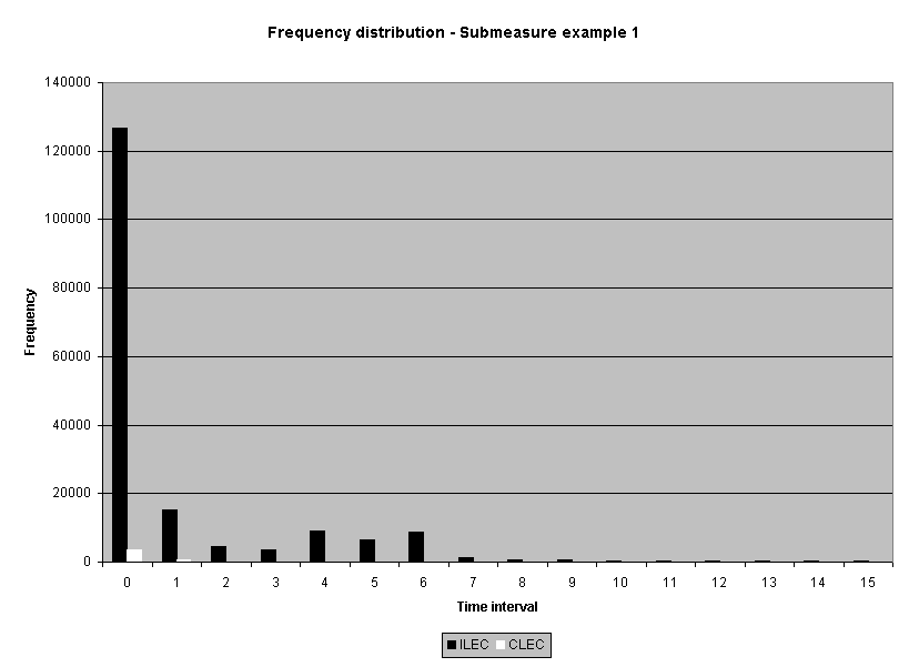
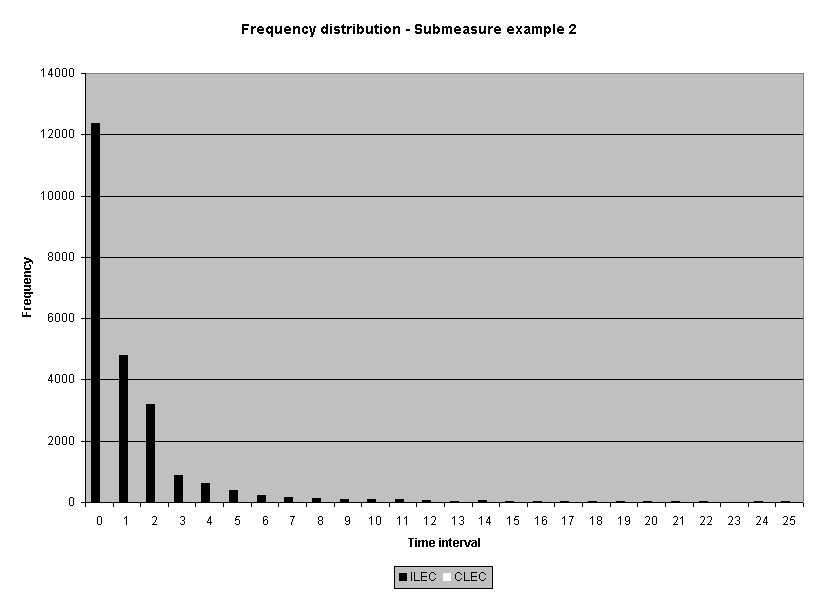
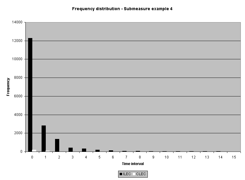
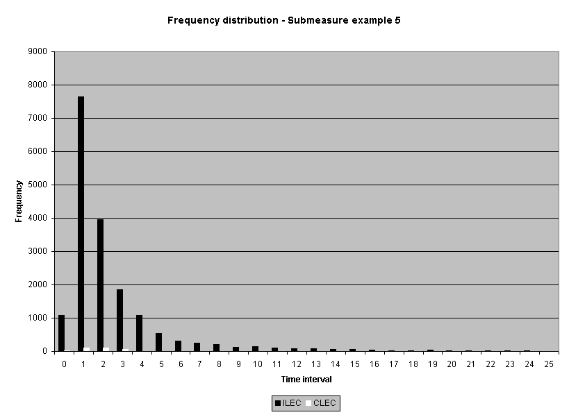
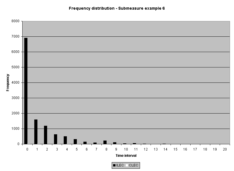
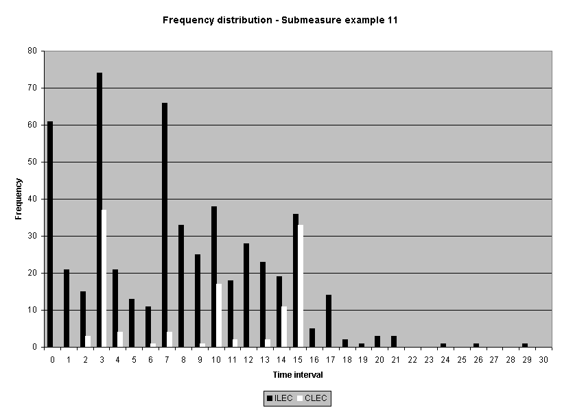
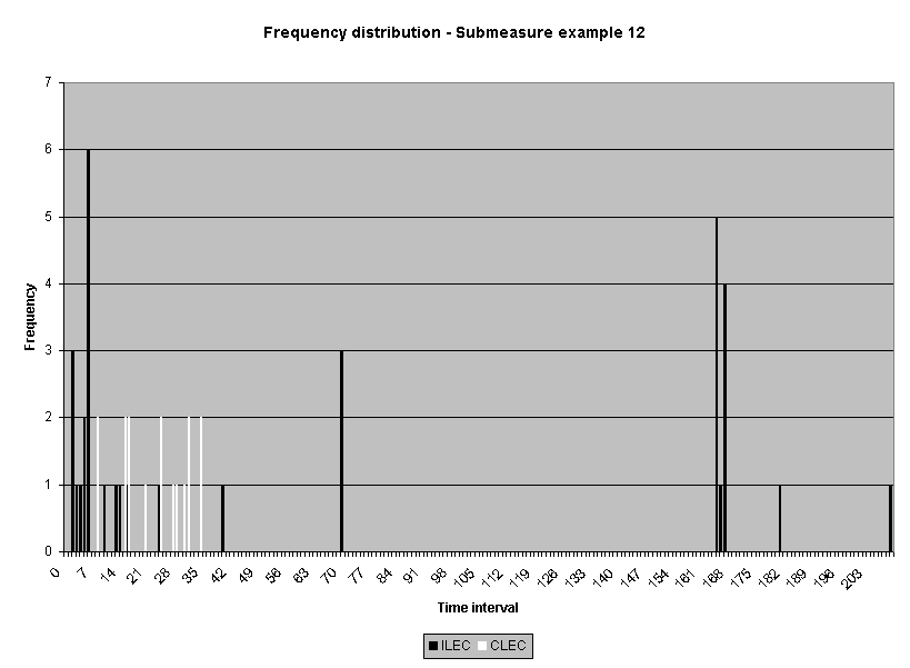
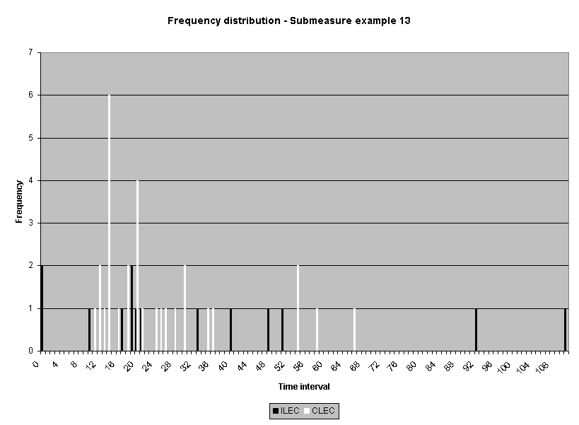
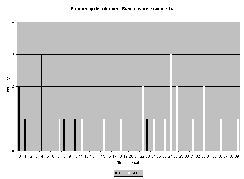
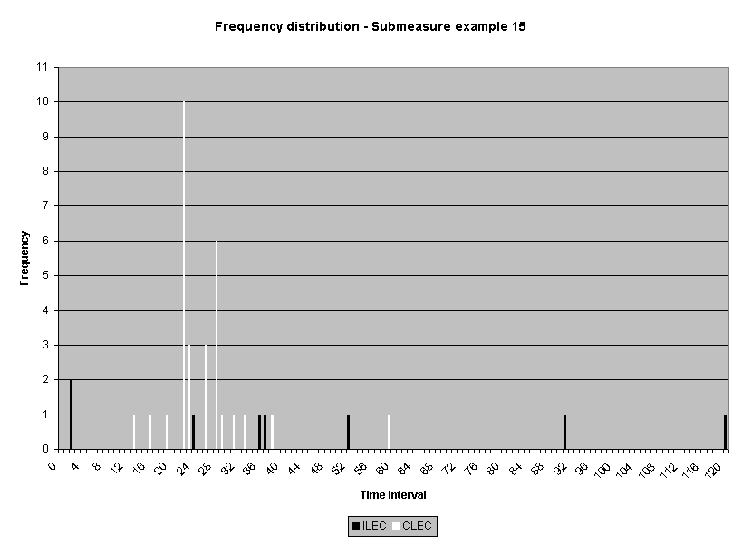
Sixteen average-based ILEC performance submeasure distributions from one performance measure were examined.⁴ Statistics for non-normality, skewness and kurtosis, were calculated. All but one of the distributions were positively skewed⁵ and all but two were leptokurtic. ⁶ While a normal curve has skeweness and kurtosis values of zero, the skewness of the sixteen submeasures ranged from 0.0 to 28.3, and the kurtosis ranged from -1.6 to 1746. Table 1 reports the skewness and kurtosis for the sixteen distributions. The frequency distribution graphs for these sixteen distributions are presented in Attachment 1 to this appendix.

Table 1

Submeasure	N	Mean	Median	Skewness	Kurtosis
Ex. 1	179254	1.18	0	21.0	1430.3
Ex. 2	23608	1.60	0	15.4	503.0
Ex. 3	19943	6.91	6	12.1	271.2
Ex. 4	17951	0.92	0	28.3	1745.7
Ex. 5	17940	2.76	2	15.6	590.3
Ex. 6	11864	1.40	0	9.1	184.6
Ex. 7	9149	1.29	0	19.7	661.2
Ex. 8	6827	2.48	1	10.3	198.6
Ex. 9	6340	3.05	1	5.3	48.2
Ex. 10	771	8.18	7	6.9	105.3
Ex. 11	538	7.89	7	1.8	8.2
Ex. 12	34	71.62	20	0.5	-1.6
Ex. 13	14	34.36	20.5	1.4	1.5
Ex. 14	9	6.00	4	1.9	4.0
Ex. 15	8	47.50	40.5	0.7	-0.1
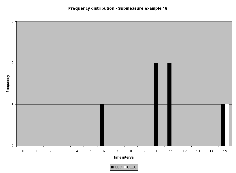
Ex. 16	6	10.50	10.5	0.0	2.1

Academic theory indicates data from measures of time to complete a task are lognormally distributed.⁷ Overall, the skewness and kurtosis of these distributions were consistent with what would be expected from a lognormal distribution. Only three of the five smallest samples (n < 35) had skewness less than one (< 1). Only two of the smallest five samples had kurtosis less than one (< 1).

Theoretical sampling mean distributions

To examine the extent of the problem posed by the skewness of the data, simulated distributions were examined to investigate the sample sizes necessary to achieve normality in the sampling mean distribution. While Central Limit Theorem poses that sampling mean distributions will be normal for many large non-normal samples, it is not clear if Central Limit Theorem's general tenet applies to the data for these measures.

At staff's request, Pacific Bell's consultant, Dr. Gleason, created a MathCad© worksheet to generate multiple samples from a lognormal distribution. This worksheet is included as Attachment 2. Using this worksheet five analyses were repeated for several selected performance results. The analysis summary following the worksheet pages shows that even for samples as large as 1000, many distributions are non-normal, the degree of departure from normality can be highly variable, and the log transformation notably improves normality.

Transformation statistical effects

Since measures of time to complete a task are theoretically lognormally distributed, log transformations of the raw data were examined. However, since the data contains values of zero (0), logs cannot be taken directly from the raw data, since the log of zero (0) cannot be computed. One recommendation is to add a constant of one (1) to each score.⁸ However, in several cases of performance measures, the raw data is actually categorized continuous data where all orders, for example, completed in the same day as initiated were assigned a zero. In these cases there are no "true" zero values since each order takes some time to complete. The lower bound of each interval is taken as the performance result, leaving the lowest interval with a value of zero.

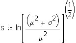
Suggesting that some value in the middle of the interval defined by each integer may be a more appropriate representation of the interval, staff asked Dr. Gleason to determine the optimal constant for the transformation. Dr. Gleason simulated continuous lognormal distributions which he then categorized using the performance data categories. Using a MathCad© worksheet (Attachment 3 to this appendix), Dr. Gleason then

calculated a constant that, when added to the actual categorized data, would best represent the parameters of the original continuous distribution. Staff used Dr. Gleason's worksheet to calculate the constant that would best fit actual ILEC and CLEC performance.9 The worksheet calculates that the upper limit for the optimal constant is approximately 0.5, with virtually all values between 0.3 and 0.5.10 The mean and standard deviation of the distributions affect the value of the constant, making the optimal constant slightly different for each analysis.

These results are theoretically reasonable as well. The mathematical midpoint of an interval in a skewed distribution¹¹ is not likely to accurately represent the distribution of scores in most intervals.

The sixteen distributions were then log-transformed using three different constants: 0.3, 0.4, and 0.5. The preponderance of transformations resulted in a closer approximation to normality. The results are presented in Attachment 4. In a few of the small samples where transformations did not improve normality, the transformed results are still relatively close to normality. From these transformations it is difficult to tell which constant best and most consistently improved normality. The transformations made with the constant of 0.5 improved normality most for large means, and the transformation with the constant of 0.3 improved normality most for the samples with small means.

Since it would be impractical to calculate the optimal constant for each result, and one of the constants must be selected, staff examined the sensitivity of the modified t-test to the different transformations. Staff sought to determine which one of the constants would result in the least discrepancy compared to using an optimal constant for each result. Type I error probabilities (_) were calculated for the sixteen submeasures. Attachment 5 presents a comparison of t-test results using raw scores and different log transformations. Use of the 0.4 constant for all results appears to minimize potential discrepancies between using result-specific optimal constants versus using a single constant for all results. In other words, compared to using the 0.3 or 0.5 constants for all results, using the 0.4 constant results in an _ closer to the _ calculated by using the result-specific optimal constant.

The constant should be added wherever the average-based performance measures produce zeros by categorizing continuous data. Following this criterion, current information indicates that constants should be used with transformations for performance measures 7, 14, 21, 28, and 37, and that performance measures 1 and 44 need no constants.

The constant should be added at the level of categorization. For example, if the smallest measurement unit is one day, then a constant of 0.4 days should be added to each observation. If the smallest measurement unit is one-hundredth of an hour, such as for performance measure 21, then the constant of 0.4 of one-hundredth (4 thousandths) of an hour should be added to each observation.

Performance evaluation implications

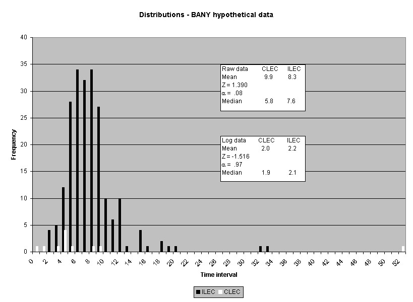
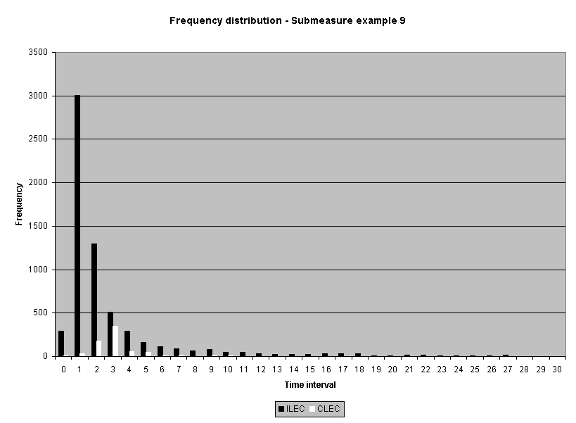
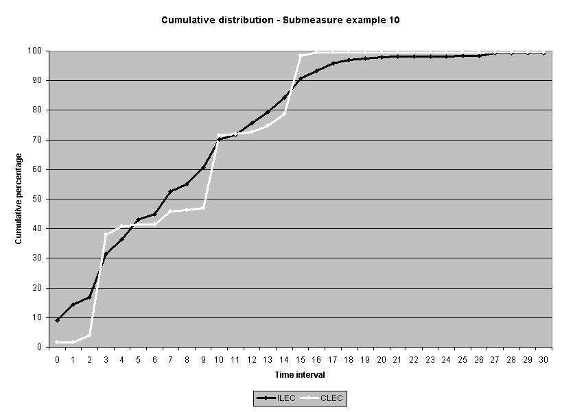
The meaning of the impact on actual performance result decisions was also examined. (See Attachment 5.) Fourteen of the 16 industry-aggregate results had the same "pass/failure" designation for the log transformation analysis as they did for the original raw score analysis. Two results failed the log-based analysis when they originally passed the raw score analysis: submeasure examples "9" and "10." Both showed CLEC average performance worse than ILEC average performance, but the average differences were not statistically different using a raw score based test. Submeasure example "9" illustrates the nature of this failure. The original data analysis resulted in a "pass" with an alpha of 0.32, whereas the log transformed data resulted in a "failure" with an alpha of less than 0.0001. For both submeasure examples "9" and "10," compared to the means, the medians showed greater differences between ILEC and CLEC performance. In these instances, the log transformation has the effect of giving a better reflection of the difference between the two distributions

than was the case for the raw data. In the raw data analyses, extreme scores in the ILEC distribution mask the typically poorer performance for the CLEC. The transformation minimizes the effects of these extreme values.

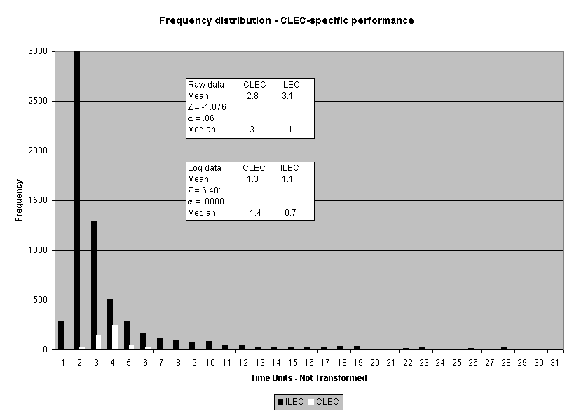
Possibly the best illustration of the difference between the log and raw score based analyses is the results for one CLEC-specific result in submeasure example "9," where the direction of the difference between the medians was the opposite for the means. Whereas the raw score CLEC mean was 2.8 days, compared to the ILEC mean of 3.0 days, the CLEC median was 3.0 and the ILEC mean was 1.0. In other words, the average time to complete the OSS task for the CLEC was 2.8 days, which is better than the 3.0-day average for the ILEC. In contrast, the median for the ILEC performance was one day while the median for the CLEC performance was two days. In other words, the ILEC took one day or less to complete the OSS task for fifty percent of its customers, whereas the ILEC took three days or less to complete the same OSS task for fifty percent of the CLECs' customers. Similar to the submeasure "9" and "10" aggregate results, the median difference for this CLEC result was much larger than the mean difference. These results show that the distributions are markedly different. Whereas the raw score analysis did not show this result to be significant (_ = 0.86), the transformation analysis identified a significant difference (_ < 0.0001).¹²

In these cases, the log transformation analysis appears to track the differences in medians more closely than the means. This is consistent with academic sources that point out the value of median-based assessments when the data is skewed. For example, Hays (1997) states,

The alteration of the score for a single extreme case in a distribution may have a profound effect on the mean. It is evident that the mean follows the skewed tail in the distribution, but the median does so to a lesser extent. The occurrence of even a few very high or very low cases can seriously distort the impression of the distribution given by the mean, provided that one mistakenly interprets the mean as the typical value. If you are dealing with a nonsymmetric distribution and you want to communicate the typical value, you must report the median. (p. 181)

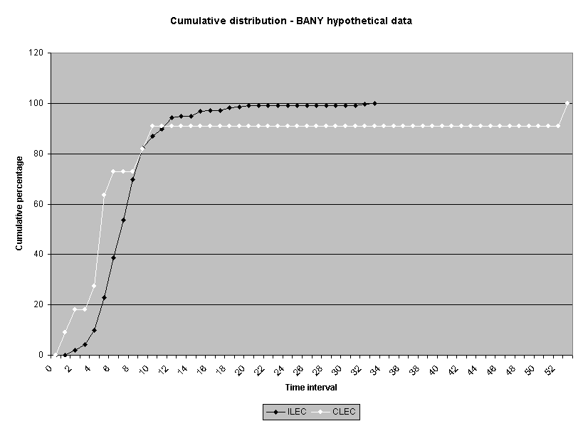
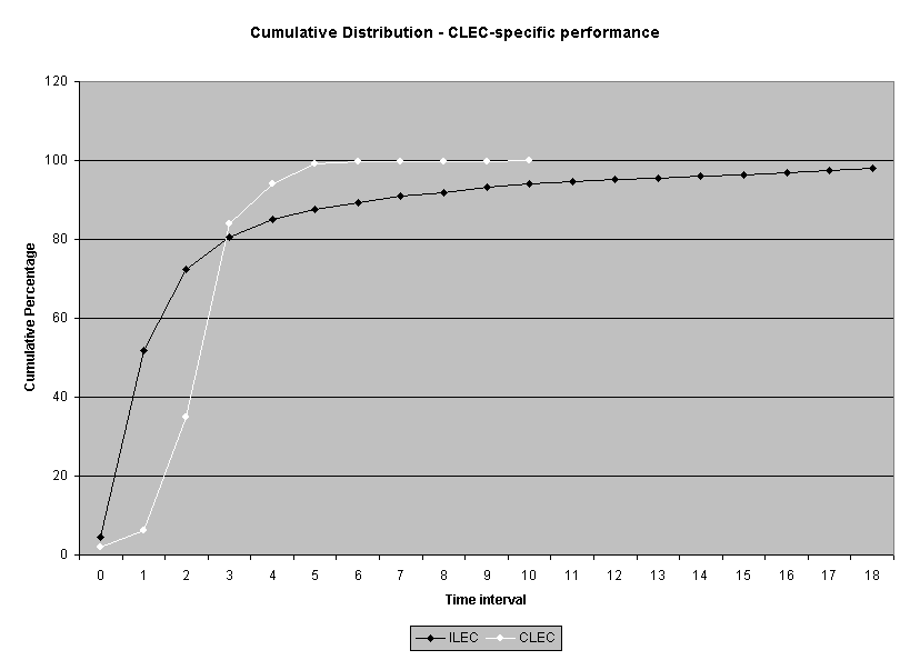
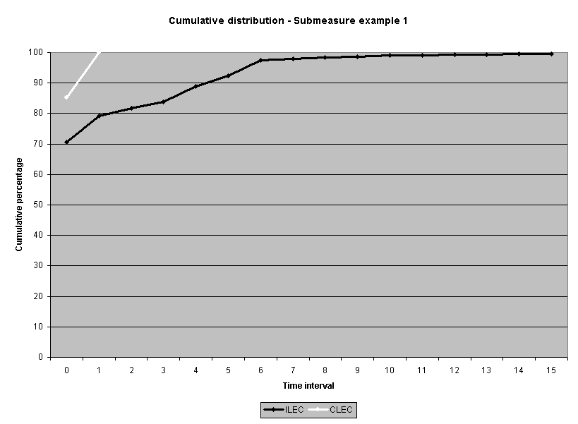
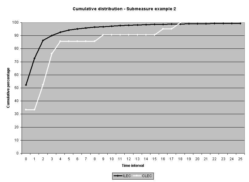
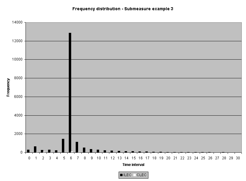
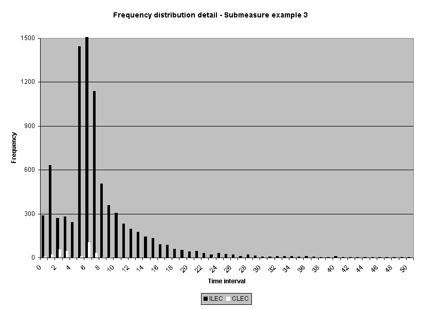
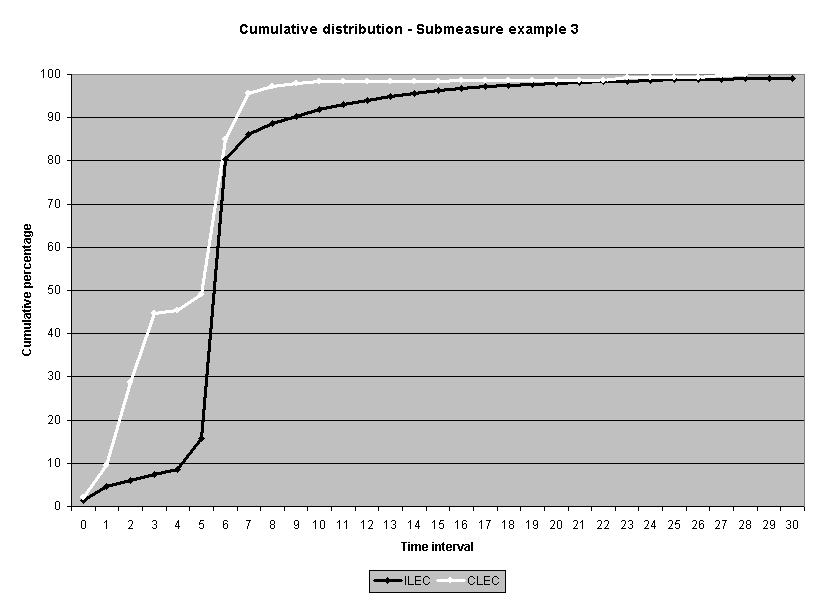
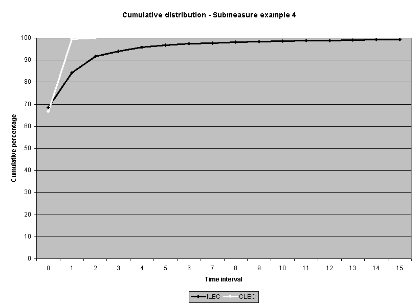
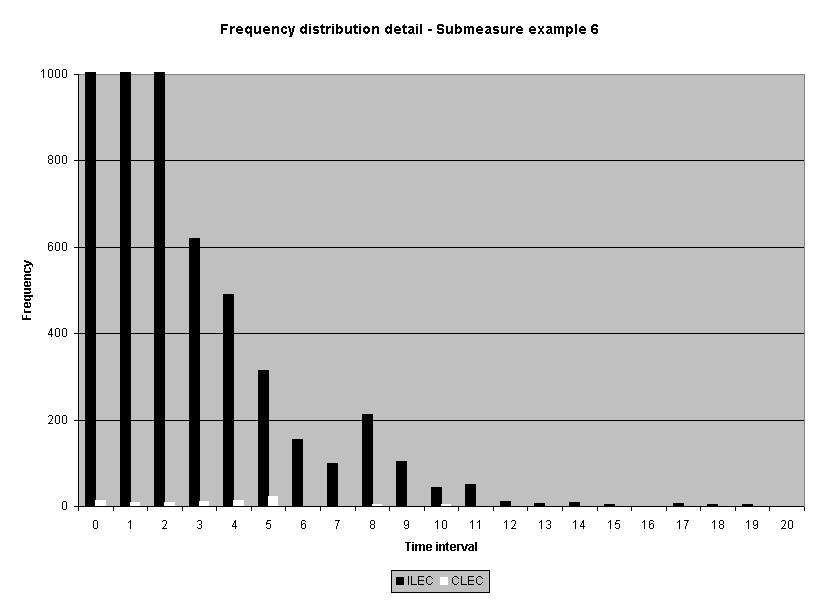
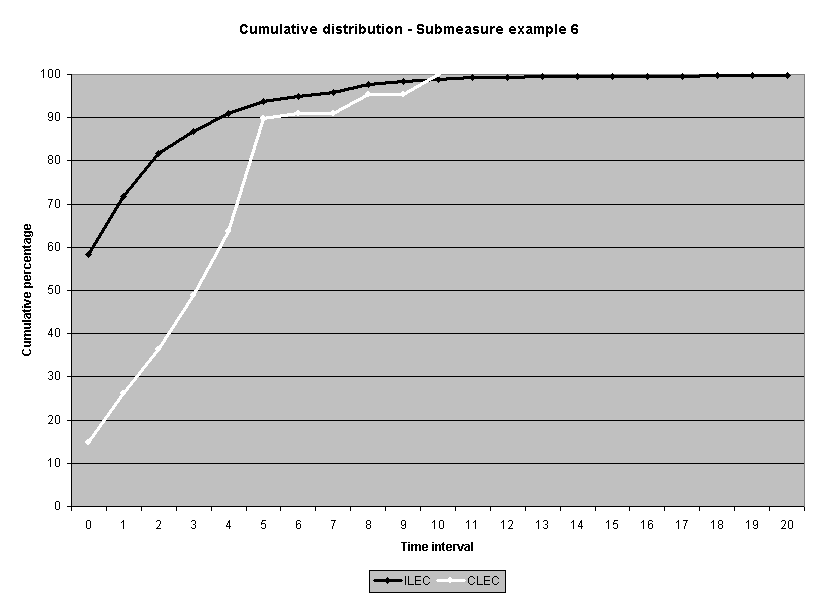
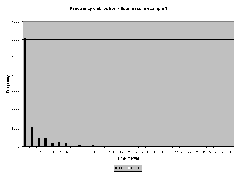
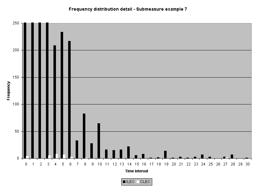
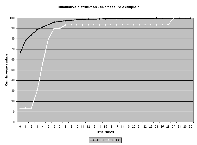
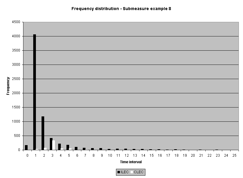
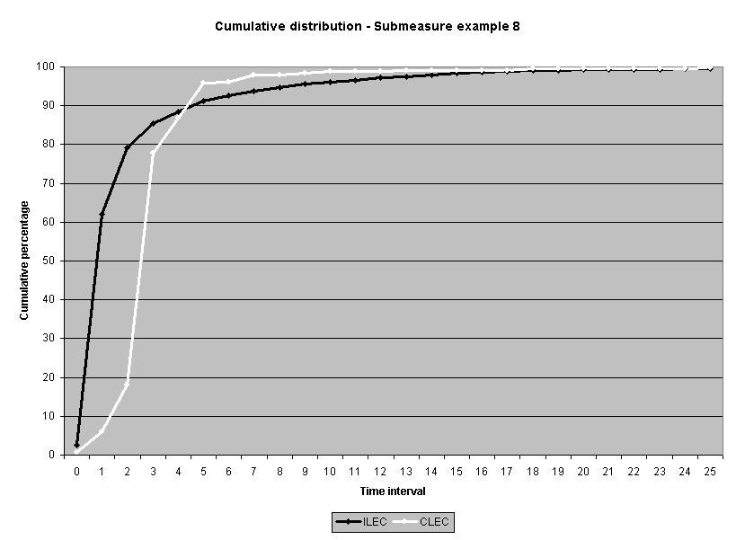
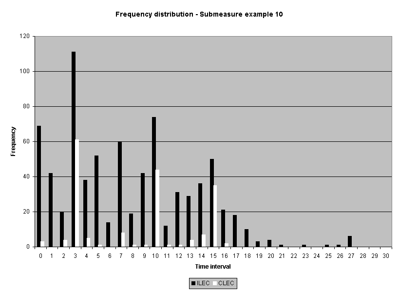
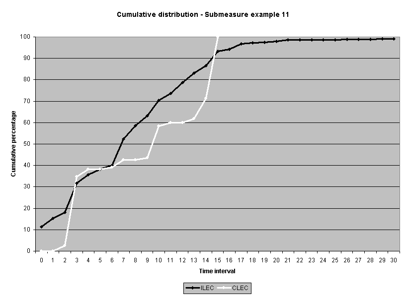
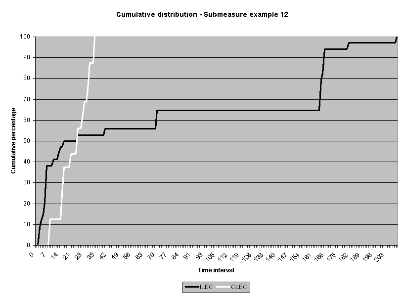
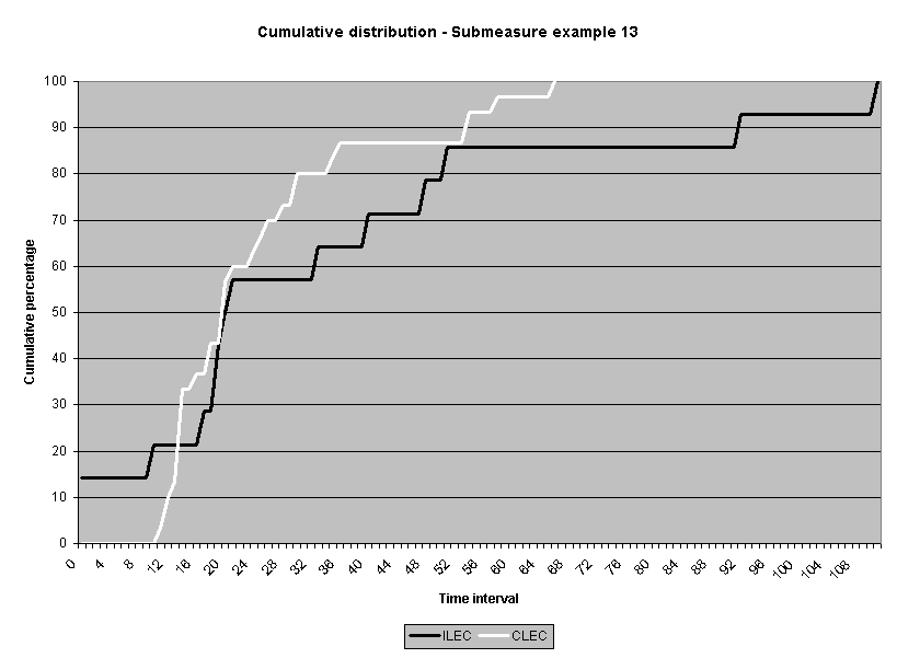
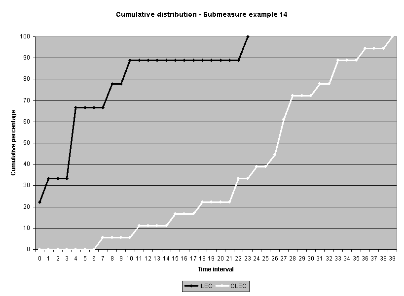
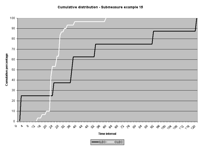
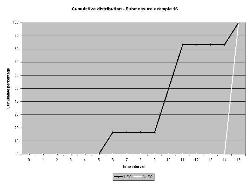
To assess the operational meaning of the transformation staff also examined the cumulative distribution. The cumulative percentage distribution data and graphs are included in Attachment 1 for submeasures 1 through 16, and in Attachment 7 for the CLEC-specific results described above. While a frequency distribution shows the number of "orders" completed for each time interval, a cumulative distribution shows the percentage of "orders" that were completed by a specific number of "days" or less.¹³ For example, the frequency distribution for submeasure "9" shows that approximately 500 of the ILEC's orders took 3 days to complete. In contrast, the cumulative distribution for submeasure "9" shows that about 80 percent of the ILEC's orders were completed in three days or less. In the cumulative distribution graphs, the higher line represents better service. For example, for submeasure "9," ILEC customers (black line) are getting better service than CLEC customers (white line) up until the point where approximately 80 percent of the orders have been completed - at a time interval of "3." Where the ILEC line is higher means that compared to CLEC customers, a greater percentage of ILEC customers are getting their orders completed within the specified time intervals. After this point, CLEC customers are getting better service as illustrated by the lines crossing. After this point the CLEC line is higher, meaning that a higher percentage of CLEC customers are getting their "orders" completed within the same time interval as ILEC customers.

The graphs in these two attachments provide a more detailed comparison of the two distributions and illustrate what the log transformation analysis detects that the raw score analysis does not. The graph shows that for submeasure example "9," for up to 80 percent of the customers, the ILEC gave better performance to its own customers. Specifically, 52 percent of ILEC customers' orders, compared to 6 percent of CLEC customers' orders, were completed within one day after the order was confirmed. Similarly, 72 percent of ILEC customers' orders, compared to 31 percent of CLEC customers' orders, were completed within two days after the order was confirmed. It is only in the final 20 percent of the distributions that CLEC customers received better performance than did the ILEC customers. For example, by the time five days passed, 88 percent of ILEC customers' orders were completed compared to 95 percent of CLEC customer's orders. These graphs depict distributions that are not "substantially equal," where CLEC customers are predominately disadvantaged even though, on the average, their completion interval is less.

Conclusions

The log transformation of time measurement raw scores that have been increased by a constant is academically supported for average-based parity measures of time to complete a task. Using a constant of 0.4 (of the smallest interval) for each transformation reasonably corrects for distribution distortions introduced by categorizing all continuous values into integers, brings the data close to being normally distributed, and results in the least variation in a Type I error probability calculation compared to using a different constant for each transformation. Additionally, sample mean distribution normality is improved not only for small to moderate samples, but also for large samples. For these reasons, this log transformation of scores with an added constant of 0.4 is the best practical option for applying the modified t-test to average-based parity measures. Additionally, the log transformation allows an appropriate statistical and practically meaningful performance assessment. Until other methods are shown to be superior and ready to implement, the Modified t-test application using log transformations is justifiable and reasonable.

References

John D. Jackson, Using permutation tests to evaluate the significance of CLEC vs. ILEC service quality differentials, Verizon CA Opening Brief, Attachment 1 at Appendix 2 (April 28, 2000).

McNemar, Q. (1962). Psychological statistics. New York: John Wiley & Sons.

Winer, B.J. (1971). Statistical principles in experimental design. New York: McGraw-Hill.

Mathcad worksheet: Investigation of the mean, standard deviation, skewness, and kurtosis of the sampling distribution of the mean before and after log transformations.

Set the parameters for the original process

Process mean

Process standard deviation

Set sample sizes

Sample size

Set additive constant for categorized distribution

Additive constant

This simulation works by generating J samples of means for which the mean, standard deviation, skewness and kurtosis are calculated. This process is repeated K times and the means of the statistics on the sampling distributions are calculated.

Set number of samples for each simulation of the sampling distribution

Set number of simulations

The following calculate the log parameters of the distribution

The following function generates a log normal distribution using logl parameters.

This function generates means for four kinds of distributions:

1. lognormal

2. log of lognormal

3. categorized lognormal (into integers) with constant

4. log of categorized lognormal with constant

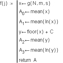
This function calculates statistics on each sample of sampling means and returns these statistics in a vector.

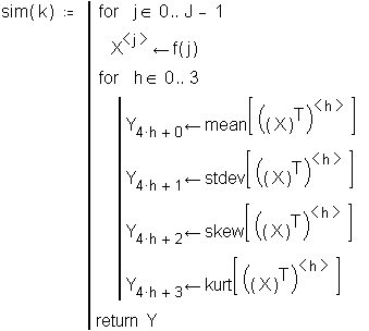
Statistics for the distribution of sample means for the untransformed (original) distribution.

Compare

Mean:

Standard Deviation:

Skewness:

Kurtosis:

Statistics for the distribution of sample means for the log transformed data.

Compare

Mean:

Standard Deviation:

Skewness:

Kurtosis:

Statistics for the distribution of sample means for the categorized data with an added constant of C.

Compare

Mean:

Standard Deviation:

Skewness:

Kurtosis:

Statistics for the distribution of sample means for the logs of the categorized data with an added constant of C.

Compare

Mean:

Standard Deviation:

Skewness:

Kurtosis:

Skewness and kurtosis variability of theoretical sampling means
	Raw data parameters				Sampling mean distribution
					Untransformed data		Transformed data
Sample size	SD	M	Cases	Constant	Skewness	Kurtosis	Skewness	Kurtosis
1000	2.6	0.5	24	0.3	1.7	7.1	0.1	0.2
					1.7	6.7	0.1	0.1
					1.6	5.9	0.1	-0.1
					1.6	5.9	0.1	0.0
					1.8	7.7	0.2	0.1
1000	2.5	0.8	129	0.4	0.9	2.2	0.1	-0.1
					0.7	1.1	0.2	-0.2
					0.9	1.6	0.1	0.0
					0.7	1.0	0.0	-0.1
					1.2	4.3	0.1	0.3
100	2.5	0.8	129	0.4	1.8	7.0	0.2	0.1
					1.7	5.3	0.2	0.1
					1.8	6.1	0.3	0.0
					2.1	9.0	0.2	0.1
					1.6	5.0	0.2	0.0
1000	6	2.9	70	0.5	0.3	0.4	-0.1	-0.2
					0.5	0.8	0.0	-0.1
					0.4	0.5	-0.1	0.0
					0.9	3.5	0.1	-0.1
					0.5	0.5	0.0	-0.1
100	6	2.9	70	0.5	1.4	4.9	0.1	0.0
					0.9	1.4	0.2	-0.2
					3.1	34.3	0.1	0.0
					1.7	8.9	0.0	0.1
					2.6	24.1	0.0	0.5
100	7	6	131	0.5	0.6	0.7	0.0	0.2
					0.6	1.1	0.1	-0.1
					0.4	0.3	0.0	0.1
					0.3	0.0	-0.1	0.0
					0.6	1.1	-0.1	0.1
30	7	6	131	0.5	1.2	3.3	0.0	0.0
					0.9	1.5	0.0	-0.1
					1.0	2.2	-0.1	-0.2
					1.1	2.3	0.0	-0.2
					0.8	1.1	-0.1	0.2
1000	16	3.1	24	0.4	1.0	1.9	0.0	-0.2
					3.2	32.2	0.0	-0.1
					1.5	4.3	0.1	0.4
					1.3	3.0	0.0	0.0
					1.6	7.1	-0.1	0.1
100	25	13	29	0.5	0.9	1.5	0.0	-0.2
					2.0	11.4	0.0	0.1
					0.9	1.6	0.1	0.6
					1.1	2.3	0.1	0.3
					1.1	3.0	-0.1	0.0

Mathcad worksheet: Investigation of the added constant used with the log transformation on a categorized lognormal distribution

Set the parameters for the original process

Process mean

Process standard deviation

Set size of sample for investigating distribution

The following calculate the log parameters of the distribution

The following function generates a log normal distribution using log

parameters.

Theoretical mean

Emprical mean

Theoretical standard deviation

Emprical standard deviation

The following solves for a, that value which, when added to the bottom end of each interval, best recreates the emprical mean

Mean using added constant

Standard deviation using added constant

(Compare to the log parameters above)

		Skewness and kurtosis of performance result distributions
			Raw score	Log(x+0.5)	Log(x+0.4)	Log(x+0.3)
		Ex. 1
		N	179254	179254	179254	179254
		Mean	1.18	-0.1128	-0.2808	-0.4948
		Median	0	-0.6931	-0.9163	-1.204
		Skewness	21.002	1.331	1.291	1.244
		Kurtosis	1430.297	0.28	0.126	-0.046
		Ex. 2
		N	23608	23608	23608	23608
		Mean	1.6	0.1008	-3.81E-02	-0.2122
		Median	0	-0.6931	-0.9163	-1.204
		Skewness	15.411	1.053	0.942	0.817
		Kurtosis	503.008	0.71	0.3	-0.131
		Ex. 3
		N	19943	19943	19943	19943
		Mean	6.91	1.8604	1.8405	1.8193
		Median	6	1.8718	1.8563	1.8405
		Skewness	12.106	-1.27	-1.513	-1.818
		Kurtosis	271.231	9.202	9.945	11.092
		Ex. 4
		N	17951	17951	17951	17951
		Mean	0.9215	-0.1906	-0.3589	-0.5723
		Median	0	-0.6931	-0.9163	-1.204
		Skewness	28.256	1.634	1.528	1.412
		Kurtosis	1745.695	2.331	1.773	1.188
		Ex. 5
		N	17940	17940	17940	17940
		Mean	2.76	0.8407	0.783	0.7187
		Median	2	0.9163	0.8755	0.8329
		Skewness	15.569	0.666	0.499	0.278
		Kurtosis	590.337	1.57	1.473	1.453
		Ex. 6
		N	11864	11864	11864	11864
		Mean	1.3988	5.55E-02	-9.15E-02	-0.277
		Median	0	-0.6931	-0.9163	-1.204
		Skewness	9.105	0.925	0.861	0.789
		Kurtosis	184.585	-0.336	-0.538	-0.755

		Skewness and kurtosis of performance result distributions
		Ex. 7
		N	9149	9149	9149	9149
		Mean	1.2922	-8.06E-02	-0.2426	-0.4484
		Median	0	-0.6931	-0.9163	-1.204
		Skewness	19.716	1.362	1.289	1.208
		Kurtosis	661.21	0.903	0.585	0.246
		Ex. 8
		N	6827	6827	6827	6827
		Mean	2.4837	0.7652	0.7077	0.6453
		Median	1	0.4055	0.3365	0.2624
		Skewness	10.337	1.493	1.364	1.187
		Kurtosis	198.575	3.221	3.021	2.868
		Ex. 9
		N	6340	6340	6340	6340
		Mean	3.05	0.8676	0.8113	0.7491
		Median	1	0.4055	0.3365	0.2624
		Skewness	5.295	0.993	0.855	0.668
		Kurtosis	48.225	1.505	1.414	1.377
		Ex. 10
		N	771	771	771	771
		Mean	8.18	1.7666	1.7302	1.6875
		Median	7	2.0149	2.0015	1.9879
		Skewness	6.917	-0.998	-1.094	-1.214
		Kurtosis	105.315	0.542	0.749	1.03
		Ex. 11
		N	538	538	538	538
		Mean	7.89	1.7286	1.6883	1.6402
		Median	7	2.0149	2.0015	1.9879
		Skewness	1.81	-1.096	-1.177	-1.277
		Kurtosis	8.242	0.408	0.579	0.802
		Ex. 12
		N	34	34	34	34
		Mean	71.6176	3.2922	3.2818	3.2712
		Median	20	3.001	2.9959	2.9908
		Skewness	0.525	-0.017	-0.023	-0.03
		Kurtosis	-1.623	-1.712	-1.705	-1.698

		Skewness and kurtosis of performance result distributions
		Ex. 13
		N	14	14	14	14
		Mean	34.3571	2.8667	2.8315	2.7871
		Median	20.5	3.0442	3.0395	3.0347
		Skewness	1.389	-1.54	-1.597	-1.664
		Kurtosis	1.484	1.906	2.033	2.184
		Ex. 14
		N	9	9	9	9
		Mean	6	1.2422	1.1746	1.0919
		Median	4	1.5041	1.4816	1.4586
		Skewness	1.874	-0.407	-0.492	-0.594
		Kurtosis	3.97	-0.763	-0.73	-0.671
		Ex. 15
		N	8	8	8	8
		Mean	47.5	3.244	3.2322	3.2201
		Median	40.5	3.7135	3.7111	3.7086
		Skewness	0.732	-1.041	-1.048	-1.056
		Kurtosis	-0.114	-0.426	-0.419	-0.412
		Ex. 16
		N	6	6	6	6
		Mean	10.5	2.3667	2.3569	2.347
		Median	10.5	2.3969	2.3877	2.3785
		Skewness	0	-0.912	-0.92	-0.929
		Kurtosis	2.086	2.601	2.611	2.62

Sensitivity analysis: Effects of transformations on alpha estimates
Ex. No.	Constant used	Ni	Mi	SDi	Nc	Mc	Z	_	Theoretical constant
1	no trnsfmn	179254	1.18	2.97	4296	0.149	-22.485	1.00
1	0.5	179254	-0.1128	0.9696	4296	-0.5295	-27.837	1.00
1	0.4	179254	-0.2808	1.0537	4296	-0.7297	-27.594	1.00	0.44
1	0.3	179254	-0.4948	1.653	4296	-0.9855	-19.228	1.00
2	no trnsfmn	23608	1.6	4.8	21	3.52	1.832	0.0335
2	0.5	23608	0.1008	0.9636	21	0.7646	3.155	0.0008	0.48
2	0.4	23608	-0.0381	1.0474	21	0.6724	3.107	0.0009
2	0.3	23608	-0.2122	1.1602	21	0.558	3.041	0.0012
4	no trnsfmn	17951	0.9215	3.4631	276	0.337	-2.783	0.997
4	0.5	17951	-0.1906	0.8292	276	-0.3251	-2.674	0.996
4	0.4	17951	-0.3589	0.907	276	-0.4968	-2.507	0.994	0.36
4	0.3	17951	-0.5723	1.012	276	-0.7131	-2.294	0.989
5	no trnsfmn	17940	2.76	4.69	302	1.755	-3.693	0.9999
5	0.5	17940	0.8407	0.739	302	0.6969	-3.353	0.9996	0.50
5	0.4	17940	0.783	0.7783	302	0.6348	-3.282	0.9995
5	0.3	17940	0.7147	0.8282	302	0.5651	-3.113	0.9991
7	no trnsfmn	9149	1.2922	4.3519	30	5.4	5.162	0.00000013
7	0.5	9149	-0.08056	0.9588	30	1.3947	8.414	0.00000000	0.40
7	0.4	9149	-0.2426	1.0421	30	1.3477	8.345	0.00000000
7	0.3	9149	-0.4484	1.1535	30	1.2916	8.249	0.00000000
9	no trnsfmn	6340	3.05	4.9	714	3.1387	0.459	0.32
9	0.5	6340	0.8676	0.782	714	1.1988	10.729	0.00	0.50
9	0.4	6340	0.8113	0.8171	714	1.1639	10.932	0.00
9	0.3	6340	0.7491	0.8608	714	1.1269	11.118	0.00
10	no trnsfmn	771	8.18	7.95	179	8.45	0.409	0.341
10	0.5	771	1.7666	1.0351	179	1.96	2.252	0.012	0.50
10	0.4	771	1.7302	1.0883	179	1.9397	2.320	0.010
10	0.3	771	1.6875	1.1571	179	1.9181	2.402	0.008
11	no trnsfmn	538	7.89	6.33	115	9.0696	1.814	0.0351
11	0.5	538	1.7286	1.0742	115	2.0628	3.028	0.0013	0.50
11	0.4	538	1.6883	1.1347	115	2.0468	3.075	0.0011
11	0.3	538	1.6402	1.2133	115	2.0303	3.130	0.0009

Ex. No.	Constant used	Ni	Mi	SDi	Nc	Mc	Z	_	Theoretical constant
13	no trnsfmn	14	34.3571	32.5874	30	25.03	-0.884	0.80
13	0.5	14	2.8667	1.6447	30	3.1086	0.454	0.33	0.50
13	0.4	14	2.8315	1.7188	30	3.1037	0.489	0.32
13	0.3	14	2.7871	1.8152	30	3.0987	0.530	0.30
14	no trnsfmn	9	6	7.2284	18	25.2222	6.514	0.00009
14	0.5	9	1.2422	1.3276	18	3.1782	3.572	0.00364	0.50
14	0.4	9	1.1746	1.4104	18	3.1736	3.472	0.00421
14	0.3	9	1.0919	1.5187	18	3.1689	3.350	0.00504
15	no trnsfmn	8	47.5	41.127	30	25.77	-1.328	0.887
15	0.5	8	3.244	1.5084	30	3.2332	-0.018	0.507	0.50
15	0.4	8	3.2322	1.5258	30	3.2291	-0.005	0.502
15	0.3	8	3.2201	1.5439	30	3.225	0.008	0.497